
Statistics · Bayesian and computational
Bootstrap Methods and Resampling
How the bootstrap uses the data themselves to measure uncertainty for medians, ratios and model outputs, which intervals to trust, how to adapt it to surveys, and where it fails.
Every estimate drawn from a sample comes with uncertainty, and reporting that uncertainty usually requires a formula for the standard error. For a mean or a simple proportion the formula is familiar. For a median basket value, a ratio of two averages, a Net Promoter Score, the importance weight of a driver or the difference between two segment medians, a convenient formula may not exist, or may rest on assumptions the data clearly break.
The bootstrap, introduced by Efron (1979), replaces the missing formula with computation. It treats the observed sample as a stand-in for the population, draws many new samples from it, recomputes the statistic each time and uses the variation among those recomputed values to measure uncertainty. The name comes from the phrase "pulling yourself up by your bootstraps": the data are used to assess their own reliability. Four decades on, the bootstrap is one of the most widely used tools in applied statistics (Efron & Hastie, 2016).
The plug-in idea
In theory, the sampling distribution of a statistic describes how it would vary if we could repeat the whole study many times. We cannot repeat the study, but we can imitate it. The bootstrap rests on the plug-in principle: if the sample is a fair picture of the population, then drawing samples from the sample mimics drawing samples from the population (Efron & Tibshirani, 1994).
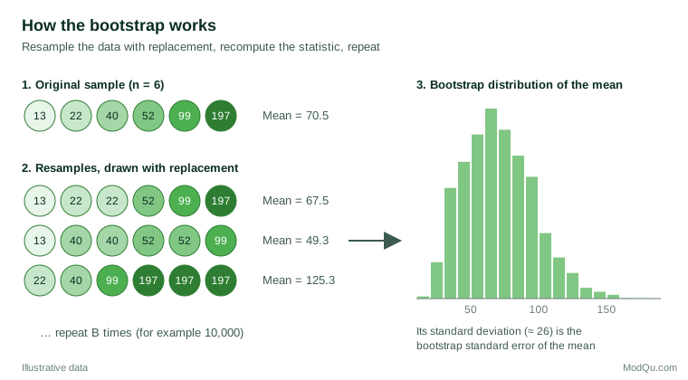
The basic, nonparametric bootstrap has four steps:
- Take the original sample of n observations.
- Draw a resample of size n with replacement, so that some observations appear more than once and others not at all. On average, a resample contains about 63% of the distinct original observations.
- Compute the statistic of interest on the resample.
- Repeat steps 2 and 3 B times, for example 10,000, and examine the B recomputed values.
The collection of recomputed values is the bootstrap distribution. Its standard deviation estimates the standard error:
SEboot = √[ Σ (θ̂*b − θ̄*)² ÷ (B − 1) ]
where θ̂b is the statistic in resample b and θ̄ is the average across resamples. The difference between θ̄* and the original estimate gives a rough measure of bias. Efron and Tibshirani (1986) set out these calculations with worked examples, and where a textbook formula exists the bootstrap answer is typically close to it.
A worked example: customer spend
Suppose, hypothetically, that a retailer surveys 40 customers about their monthly spend. As is typical for spending data, the distribution is skewed: most customers spend between $15 and $100, but a few spend $200 to $300. The sample mean is $74.38, the standard deviation is $68.11 and the median is $51.50.
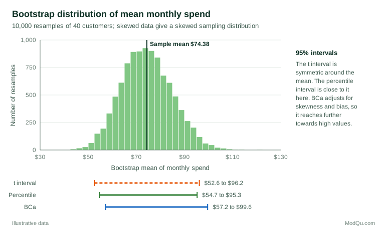
For the mean, the usual formula gives a standard error of $68.11 ÷ √40 = $10.77. Running 10,000 bootstrap resamples gives a standard error of $10.44, very close, as we would expect. The bootstrap distribution of the mean (Figure 2) is visibly skewed to the right, because the occasional resample that includes several big spenders pulls the mean up sharply.
For the median there is no simple textbook formula that works well in a sample this size. The bootstrap answers the question directly: the standard error of the median is about $8.84, and the middle 95% of bootstrap medians runs from $38.00 to $70.50. The same few lines of code would work for a trimmed mean, the share spending more than $100, or the ratio of spend to visit frequency.
Bootstrap confidence intervals
A standard error is useful, but decision-makers usually want a confidence interval. Several bootstrap intervals exist, and they differ in accuracy (DiCiccio & Efron, 1996).
| Method | How it works | Strengths and weaknesses |
|---|---|---|
| Normal | Estimate ± 1.96 × SEboot | Simple; assumes a symmetric, bell-shaped distribution |
| Percentile | 2.5th and 97.5th percentiles of the bootstrap distribution | Intuitive and respects skew; too narrow in small samples |
| Bootstrap-t | Resamples a standardised statistic | Accurate when a good standard error is available for each resample |
| BCa | Percentiles adjusted for bias and skewness | Good general-purpose choice; needs more resamples |
The bias-corrected and accelerated (BCa) interval, proposed by Efron (1987), shifts and stretches the percentile interval to correct for bias in the estimate and for a standard error that changes with the value of the parameter. Theoretical work by Hall (1992) showed that BCa and bootstrap-t intervals are "second-order accurate": their coverage errors shrink faster as the sample grows than those of normal-theory or simple percentile intervals.
In the spend example, the t interval of $52.60 to $96.20 is symmetric around the mean. The percentile interval is similar, but the BCa interval of $57.20 to $99.60 is shifted towards higher values, which better reflects the long right tail of the data. Hesterberg (2015) shows that the simple percentile interval is often too narrow in small samples and points to more accurate alternatives, such as the bootstrap-t.
How many resamples?
Early guidance suggested that 50 to 200 resamples were enough for a standard error, with 1,000 or more for confidence intervals (Efron & Tibshirani, 1994). Computing is now cheap, and Hesterberg (2015) argues for around 10,000 resamples in routine work, so that the random variation from the resampling itself is negligible. A practical check is to run the analysis twice with different random seeds; if the reported figures change in a digit that matters, increase B. Always record the seed so results can be reproduced.
Variations for different kinds of data
The basic bootstrap assumes the observations are independent and identically distributed. Real business data often are not, and the resampling scheme must mirror how the data were generated (Davison & Hinkley, 1997).
- Regression. Freedman (1981) described two approaches: resampling whole cases (rows), which is robust when error variance differs across observations, and resampling residuals, which assumes a correctly specified model with constant variance. Case resampling is the safer default for survey data.
- Time series. Resampling individual weeks of sales data destroys the dependence between neighbouring weeks. The moving block bootstrap resamples blocks of consecutive observations instead (Künsch, 1989), and the stationary bootstrap uses blocks of random length (Politis & Romano, 1994).
- Parametric bootstrap. When a model, such as a Poisson model for complaint counts, is trusted, resamples can be simulated from the fitted model rather than drawn from the data.
- Bayesian bootstrap. Rubin (1981) showed that giving each observation a random weight, rather than a random count, yields a posterior distribution under a simple nonparametric model.
- Bagging. Breiman (1996) used bootstrap resamples to build many versions of a predictive model and average them, which stabilises unstable methods such as decision trees.
Resampling complex survey data
Most commercial surveys use stratification, clustering and weighting. A naive bootstrap that resamples individual respondents ignores this design and usually understates the standard error when respondents are clustered (Lohr, 2021).
For design-based surveys, the bootstrap is applied to the primary sampling units within each stratum. Rao and Wu (1988) proposed a rescaling bootstrap that corrects the variance for the number of units drawn in each stratum, and it remains a standard approach. Many statistical agencies now publish replicate weights built from the bootstrap, the jackknife or balanced repeated replication, so that analysts can compute valid standard errors for any statistic without knowing design details (Wolter, 2007).
Two practical points matter for market researchers. First, if the weights were produced by raking or calibration to population totals, that weighting step should be repeated within each replicate; otherwise the variance contributed by weighting is missed. Second, when a panel or tracking study measures the same respondents repeatedly, the respondent, not the individual response, is the unit to resample.
Common business applications
- Medians, percentiles and ratios. Median order value, the 90th percentile of delivery time and revenue per visit all lack simple formulas; the bootstrap handles them directly.
- Indices and scores. Net Promoter Score is the difference of two proportions taken from the same respondents. Resampling respondents captures the dependence between the two proportions automatically.
- Mediation analysis. The indirect effect in a mediation model is a product of two coefficients with a skewed sampling distribution. Bootstrap intervals have become the standard way to test it (Preacher & Hayes, 2008).
- Online experiments. Metrics such as revenue per user are heavy-tailed, and ratio metrics such as click-through rate per page view need careful variance estimation. Kohavi et al. (2020) discuss the delta method and the bootstrap for estimating the variance of such metrics in A/B tests.
- Driver and segmentation stability. Resampling respondents and refitting a driver model or cluster solution shows whether importance rankings or segment memberships are stable or an accident of one sample.
Bootstrap or permutation test?
Resampling is also used for hypothesis tests, and the two ideas are easy to confuse. A permutation test shuffles group labels, for example "saw advertisement A" and "saw advertisement B", to build the distribution of a difference under the assumption that the groups do not differ. It answers a yes/no question about a null hypothesis. The bootstrap resamples within the observed data, without assuming any null, to estimate how precise a difference is. In practice, a bootstrap confidence interval for the difference in medians between two segments is usually more informative for business decisions than a permutation p-value, because it shows the size of the difference and its plausible range, not only whether it is distinguishable from zero.
Reporting bootstrap results
A short methods note makes bootstrap results credible and reproducible. State the statistic, the resampling unit (respondent, household or cluster), whether weights or strata were respected, the number of resamples, the interval method and the random seed. For example: "95% BCa confidence interval from 10,000 bootstrap resamples of respondents within strata, with weights recalculated in each resample." Showing a histogram of the bootstrap distribution, as in Figure 2, also helps readers see skew or lumpiness that a single interval hides.
When the bootstrap fails
The bootstrap is powerful but not magic. Its justification is asymptotic: it works when the sample is large enough to represent the population and the statistic is a smooth function of the data (Bickel & Freedman, 1981). Known problem cases include:
- Very small samples. With 10 observations, the bootstrap can only rearrange 10 values, and percentile intervals in particular will be too narrow.
- Extremes. The bootstrap distribution of a sample maximum or minimum is poor, because no resample can exceed the largest observed value.
- Very heavy tails. For data with extremely long tails, such as revenue from a few large clients, the bootstrap of the mean can be unreliable; trimmed means or medians may be better targets.
- Dependence ignored. Clustered, time-ordered or matched data need a resampling scheme that reflects the structure, as described above.
- Bias in the data. Resampling measures sampling variability only. It cannot correct nonresponse, coverage error or a leading question; a biased sample produces a confidently wrong bootstrap interval.
Davison and Hinkley (1997) recommend diagnostic plots of the bootstrap distribution and of each observation's influence on the result to detect these problems.
Common mistakes
- Resampling the wrong unit. Resample respondents, households or clusters as they were sampled, not individual answers.
- Using too few resamples and reporting figures more precisely than the resampling supports.
- Defaulting to the percentile interval in small or skewed samples where BCa or bootstrap-t would be more accurate.
- Reporting bootstrap results as if the bootstrap removed bias. The bias estimate is approximate, and correcting it can add noise.
- Forgetting the weights. Unweighted resampling of weighted survey data answers a different question from the one the weighted estimate answers.
Key takeaways
The bootstrap measures uncertainty by recomputing a statistic on many samples drawn from the data themselves. It frees analysts from needing a formula for every statistic, works well for medians, ratios, scores and model outputs, and is easy to explain to business audiences. Use enough resamples, prefer BCa or bootstrap-t intervals in small or skewed samples, resample in a way that matches the sampling design, and remember that the bootstrap measures random error only, not bias.
References
Bickel, P. J., & Freedman, D. A. (1981). Some asymptotic theory for the bootstrap. The Annals of Statistics, 9(6), 1196–1217. https://doi.org/10.1214/aos/1176345637
Breiman, L. (1996). Bagging predictors. Machine Learning, 24(2), 123–140. https://doi.org/10.1007/BF00058655
Davison, A. C., & Hinkley, D. V. (1997). Bootstrap methods and their application. Cambridge University Press. https://doi.org/10.1017/CBO9780511802843
DiCiccio, T. J., & Efron, B. (1996). Bootstrap confidence intervals. Statistical Science, 11(3), 189–228. https://doi.org/10.1214/ss/1032280214
Efron, B. (1979). Bootstrap methods: Another look at the jackknife. The Annals of Statistics, 7(1), 1–26. https://doi.org/10.1214/aos/1176344552
Efron, B. (1987). Better bootstrap confidence intervals. Journal of the American Statistical Association, 82(397), 171–185. https://doi.org/10.1080/01621459.1987.10478410
Efron, B., & Hastie, T. (2016). Computer age statistical inference: Algorithms, evidence, and data science. Cambridge University Press. https://doi.org/10.1017/CBO9781316576533
Efron, B., & Tibshirani, R. (1986). Bootstrap methods for standard errors, confidence intervals, and other measures of statistical accuracy. Statistical Science, 1(1), 54–75. https://doi.org/10.1214/ss/1177013815
Efron, B., & Tibshirani, R. J. (1994). An introduction to the bootstrap. Chapman and Hall/CRC. https://doi.org/10.1201/9780429246593
Freedman, D. A. (1981). Bootstrapping regression models. The Annals of Statistics, 9(6), 1218–1228. https://doi.org/10.1214/aos/1176345638
Hall, P. (1992). The bootstrap and Edgeworth expansion. Springer. https://doi.org/10.1007/978-1-4612-4384-7
Hesterberg, T. C. (2015). What teachers should know about the bootstrap: Resampling in the undergraduate statistics curriculum. The American Statistician, 69(4), 371–386. https://doi.org/10.1080/00031305.2015.1089789
Kohavi, R., Tang, D., & Xu, Y. (2020). Trustworthy online controlled experiments: A practical guide to A/B testing. Cambridge University Press. https://doi.org/10.1017/9781108653985
Künsch, H. R. (1989). The jackknife and the bootstrap for general stationary observations. The Annals of Statistics, 17(3), 1217–1241. https://doi.org/10.1214/aos/1176347265
Lohr, S. L. (2021). Sampling: Design and analysis (3rd ed.). Chapman and Hall/CRC. https://doi.org/10.1201/9780429298899
Politis, D. N., & Romano, J. P. (1994). The stationary bootstrap. Journal of the American Statistical Association, 89(428), 1303–1313. https://doi.org/10.1080/01621459.1994.10476870
Preacher, K. J., & Hayes, A. F. (2008). Asymptotic and resampling strategies for assessing and comparing indirect effects in multiple mediator models. Behavior Research Methods, 40(3), 879–891. https://doi.org/10.3758/BRM.40.3.879
Rao, J. N. K., & Wu, C. F. J. (1988). Resampling inference with complex survey data. Journal of the American Statistical Association, 83(401), 231–241. https://doi.org/10.1080/01621459.1988.10478591
Rubin, D. B. (1981). The Bayesian bootstrap. The Annals of Statistics, 9(1), 130–134. https://doi.org/10.1214/aos/1176345338
Wolter, K. M. (2007). Introduction to variance estimation (2nd ed.). Springer. https://doi.org/10.1007/978-0-387-35099-8