
Statistics · Bayesian and computational
Bayes' Theorem and Updating Beliefs With Evidence
How Bayes' theorem turns prior beliefs and new evidence into updated probabilities, shown through survey examples, with guidance on likelihood ratios, priors, credible intervals and common reasoning errors.
Every business decision rests on beliefs that should change when new evidence arrives. A product team believes a concept will appeal to about a fifth of its target market, then a concept test comes in. An analyst suspects that a respondent belongs to a particular customer segment, then sees how the respondent answered two questions. In both cases the question is the same: given what we believed before and what we have just observed, what should we believe now?
Bayes' theorem answers that question with a single, simple rule of probability. It was set out in an essay by the Reverend Thomas Bayes, published after his death by his friend Richard Price (Bayes, 1763), and developed much further by Pierre-Simon Laplace (Stigler, 1986). Today it underpins Bayesian inference, a complete approach to statistics, as well as spam filters, recommendation engines and many classification methods. This article explains what the theorem says, works through two survey examples, and discusses where prior beliefs come from, how Bayesian results differ from conventional ones, and the reasoning errors the theorem helps to avoid.
The theorem
For a hypothesis H and some evidence E, Bayes' theorem states:
P(H | E) = P(E | H) × P(H) ÷ P(E)
Each term has a name and a role:
- P(H) is the prior probability: how plausible the hypothesis was before seeing the evidence.
- P(E | H) is the likelihood: how probable the evidence would be if the hypothesis were true.
- P(E) is the overall probability of the evidence, averaged across all the hypotheses under consideration. It acts as a scaling factor that makes the updated probabilities add up to 1.
- P(H | E) is the posterior probability: how plausible the hypothesis is after taking the evidence into account.
When there are several competing hypotheses H1, H2, … Hk, the denominator is the sum of prior × likelihood across all of them:
P(E) = Σi P(E | Hi) × P(Hi)
So the recipe is always the same. Multiply each hypothesis's prior by the likelihood of the evidence under that hypothesis, then divide each product by their total. The theorem follows directly from the definition of conditional probability, so it is not controversial in itself (Blitzstein & Hwang, 2019). What is debated, as discussed below, is when and how prior probabilities should be used in statistical analysis.
Why the theorem matters: the two directions of a conditional probability
The theorem's practical value comes from the fact that P(E | H) and P(H | E) are different quantities, and people often confuse them. The probability that a loyal customer gives a high satisfaction score is not the same as the probability that a customer who gives a high score is loyal. The first is usually what we can measure or model; the second is usually what we want to know. Bayes' theorem is the bridge between the two, and the bridge always passes through the prior. If loyal customers are rare, even a strong link between loyalty and high scores may leave most high scorers not loyal.
A worked example: which segment is this respondent in?
Suppose, hypothetically, that a retailer's segmentation study has divided its customers into three segments: value seekers (50% of customers), convenience-first shoppers (30%) and premium loyalists (20%). A short screener is used to place new survey respondents into a segment. From the original study, the analyst knows how often members of each segment agree with two screener statements:
| Segment | Share of customers | Would pay extra for next-day delivery | Usually buys the store brand |
|---|---|---|---|
| Value seekers | 50% | 20% | 80% |
| Convenience-first | 30% | 70% | 40% |
| Premium loyalists | 20% | 50% | 10% |
A new respondent agrees with the first statement. Before the answer, the prior probabilities are simply the segment sizes. The likelihoods of a "yes" are 0.2, 0.7 and 0.5. Multiplying gives 0.5 × 0.2 = 0.10 for value seekers, 0.3 × 0.7 = 0.21 for convenience-first and 0.2 × 0.5 = 0.10 for premium loyalists. These add up to 0.41, the overall probability of a "yes". Dividing each product by 0.41 gives posterior probabilities of 24%, 51% and 24%. One answer has moved convenience-first from the least likely of the two larger segments to the most likely segment overall.
The respondent then says they usually buy the store brand. The posterior from the first answer now becomes the prior for the second. Multiplying by the new likelihoods (0.8, 0.4 and 0.1) and rescaling gives 46%, 48% and 6%. Premium loyalists are now very unlikely, but the respondent is almost equally likely to be a value seeker or a convenience-first shopper. Figure 1 shows the sequence.
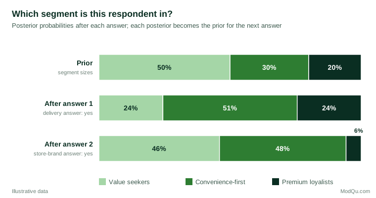
Three lessons follow. First, evidence shifts beliefs in proportion to how much more likely it is under one hypothesis than another, not in proportion to how "typical" it seems. Second, two pieces of evidence can pull in different directions, and the theorem combines them coherently. Third, the result depends on the priors: the same two answers from a respondent recruited from a list of premium-card holders, where premium loyalists might make up most of the sample, would give a quite different posterior.
This is the logic of the naive Bayes classifier and, in more elaborate form, of latent class models that assign respondents to segments with posterior membership probabilities. The word "naive" refers to the assumption that the answers are independent within each segment, which allows their likelihoods to be multiplied. If the two statements were strongly related within segments, multiplying their likelihoods would count the same evidence twice.
The odds form and the likelihood ratio
Bayes' theorem is often easier to use in its odds form. For two competing hypotheses H1 and H2:
posterior odds = prior odds × likelihood ratio
where the likelihood ratio is P(E | H1) ÷ P(E | H2). In the example, the prior odds of convenience-first against value seekers are 0.3 ÷ 0.5 = 0.6. The first answer has a likelihood ratio of 0.7 ÷ 0.2 = 3.5 in favour of convenience-first, so the odds become 0.6 × 3.5 = 2.1. The second answer has a likelihood ratio of 0.4 ÷ 0.8 = 0.5, which halves the odds to 1.05, almost even.
The odds form makes the separate contributions of the prior and the evidence explicit. The likelihood ratio is a measure of the strength of evidence that does not depend on the prior, which is why it is used to summarise diagnostic tests, forensic evidence and statistical comparisons of models. When the hypotheses are statistical models, the likelihood ratio averaged over each model's parameters is called the Bayes factor. Kass and Raftery (1995) suggested reading Bayes factors of 1 to 3 as evidence "not worth more than a bare mention", 3 to 20 as positive, 20 to 150 as strong and above 150 as very strong.
Updating step by step
The segment example shows an important property: updating one piece of evidence at a time gives the same final answer as updating on all the evidence at once, and the order does not matter, provided the pieces of evidence are conditionally independent given each hypothesis. Yesterday's posterior is today's prior. This is what makes Bayesian reasoning a natural model of learning. A brand tracker, a churn model or a sales forecast can be refreshed as each new wave of data arrives without starting again from scratch (McElreath, 2020).
It also shows that strong priors need strong evidence to overturn them. With prior odds of 1 to 99 against a hypothesis, evidence with a likelihood ratio of 10 raises the odds only to about 1 to 10. Several independent pieces of evidence of that strength would be needed to make the hypothesis more likely than not.
From hypotheses to estimates: updating a proportion
Bayes' theorem applies not only to a short list of hypotheses but also to a continuous quantity, such as the true share of target buyers who would buy a new product. In that case the prior and posterior are probability distributions across all possible values.
Suppose, hypothetically, that a food manufacturer has tested many past concepts and that their purchase-intent rates, the share saying they would definitely or probably buy, have averaged about 20% and rarely exceeded 35%. The analyst encodes this experience as a beta distribution with parameters 6 and 24, which has a mean of 20% and puts 95% of its probability between about 8% and 36%. A new concept is then tested with 120 respondents, of whom 36 (30%) express purchase intent.
The beta distribution is convenient because, combined with binomial data, it gives a beta posterior: the analyst simply adds the number of "yes" answers to the first parameter and the number of "no" answers to the second (Gelman et al., 2013). The posterior is a beta distribution with parameters 6 + 36 = 42 and 24 + 84 = 108. Its mean is 42 ÷ 150 = 28%, and a 95% credible interval runs from 21% to 35% (Figure 2).
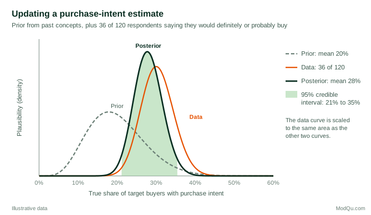
Three features of the result deserve comment. First, the posterior mean of 28% lies between the prior mean (20%) and the sample result (30%), closer to the data because the sample carries more information than the prior. The prior is worth about 30 respondents (6 + 24), while the data are worth 120. Second, the credible interval has a direct interpretation: given the prior and the data, there is a 95% probability that the true rate lies between 21% and 35%. A conventional 95% confidence interval for the sample alone, 22% to 38%, does not support that probability statement, although it is often misread as if it did. Third, the posterior answers business questions directly. The probability that the true rate exceeds a 25% launch threshold is about 79%, a figure a decision-maker can weigh against the cost of being wrong.
As data accumulate, the prior matters less. With 1,200 respondents and the same 30% result, the posterior mean would be 29.8% and the prior would make almost no difference. Edwards et al. (1963) called this the principle of stable estimation: when the data are informative, reasonable people who start from different priors end up with nearly the same conclusions.
Where priors come from
The prior is the most distinctive and most criticised part of Bayesian analysis. Critics argue that it lets personal opinion into what should be an objective analysis, and Efron (1986) noted that this concern is one of the main reasons the conventional approach has dominated scientific reporting. Supporters reply that every analysis involves judgements, about the model, the sample and the variables, and that the Bayesian approach at least makes one of them explicit and open to challenge (Lindley, 2000).
In business research, good priors are usually available and defensible:
- Historical data. Past concepts, past waves of a tracker or past campaigns provide an empirical base, as in the concept test above.
- Benchmarks and published norms. Category averages or industry studies set a plausible range.
- Expert judgement. Structured elicitation from product managers or sales teams can be turned into a distribution, as long as overconfidence is checked.
- Weakly informative priors. When little is known, priors that rule out absurd values while letting the data dominate are a common default. Gelman et al. (2017) stress that a prior can only be understood in the context of the model and data it is combined with.
Whatever the source, a sensitivity analysis, rerunning the analysis with a more optimistic and a more sceptical prior, shows how much the conclusion depends on that choice. If the decision changes, the data are not yet strong enough to settle the question on their own. Gelman and Shalizi (2013) also argue that Bayesian models should be checked against the data like any other model, rather than treated as a final statement of belief.
Bayesian and conventional statistics
Conventional, or frequentist inference, treats unknown quantities as fixed and asks how often a procedure would give a particular result over repeated samples. Bayesian inference treats unknown quantities as uncertain and describes that uncertainty with probabilities (Wasserman, 2004). The two approaches often give similar numbers, especially with large samples and weak priors, and Bayarri and Berger (2004) argue that each has much to learn from the other.
The differences matter most in three situations. First, p-values answer the question "how surprising are these data if there is no effect?", not "how likely is it that there is an effect?". Berger and Sellke (1987) showed that a p-value of 0.05 can correspond to a much higher posterior probability of no effect than 5%, so it may represent weaker evidence than many readers assume. Wagenmakers (2007) set out the problems of p-values and argued for Bayes factors as an alternative. Second, small samples benefit from prior information, which stabilises estimates for small subgroups or rare events. Third, decisions often require probability statements about the quantity itself, which only a Bayesian analysis provides. Kruschke and Liddell (2018) describe how Bayesian estimation can replace or complement conventional tests and confidence intervals in everyday research.
Bayes and human judgement
Bayes' theorem is also a benchmark for everyday reasoning, and people often fall short of it. The most studied failure is base rate neglect: judging the probability of a hypothesis by how well the evidence fits it while ignoring how common the hypothesis is in the first place. Kahneman and Tversky (1972) showed that people judge probability by representativeness, meaning resemblance to a stereotype, and Tversky and Kahneman (1974) placed this among a broader family of heuristics that produce predictable biases. Casscells et al. (1978) found that most of the medical staff and students they surveyed gave badly wrong answers to a simple screening problem: the most common answer was 95%, when the correct figure was about 2%.
The remedy is often a change of format rather than more training in formulas. Gigerenzer and Hoffrage (1995) found that people reason far more accurately when the same information is presented as natural frequencies, for example "of 1,000 customers, 300 are convenience-first, and 210 of them would pay for next-day delivery", instead of as conditional percentages. Hoffrage et al. (2000) and Gigerenzer et al. (2007) showed that the same approach helps physicians and other professionals to interpret statistical evidence. Spiegelhalter (2017) reviews wider evidence on communicating risk and uncertainty and also recommends expected frequencies. For survey reports, this means presenting conditional results as counts out of a clear reference group wherever possible.
Practical guidance for business and survey data
- State the prior and its source. Whether it comes from history, benchmarks or judgement, make it visible so that others can challenge it.
- Report the evidence strength separately. Likelihood ratios or Bayes factors show what the new data contribute, independent of the prior.
- Check independence before multiplying. Correlated pieces of evidence, such as several similar survey items, should not be treated as separate confirmations.
- Run a sensitivity analysis. Show results under a sceptical and an optimistic prior when stakes are high.
- Present posteriors as decision-ready statements. "There is a 79% probability that intent exceeds 25%" is more useful than a bare interval.
- Use natural frequencies in reports. They make conditional reasoning accessible to non-specialist readers.
Common mistakes
- Confusing P(E | H) with P(H | E). The probability of the evidence given a hypothesis is not the probability of the hypothesis given the evidence.
- Ignoring the base rate. Strong evidence about a rare hypothesis can still leave it unlikely.
- Double counting evidence. Treating related observations as independent exaggerates how much beliefs should change.
- Using overconfident priors. A prior that rules out plausible values cannot be corrected by data, since a prior probability of zero stays at zero whatever the evidence.
- Hiding the prior. An analysis whose prior is not reported cannot be assessed or reproduced.
- Reading a confidence interval as a credible interval. Only the Bayesian interval supports a direct probability statement about the true value.
Key takeaways
Bayes' theorem is the rule for learning from evidence. It combines a prior belief with the likelihood of new evidence to produce a posterior belief, and that posterior becomes the starting point for the next piece of evidence. In its odds form it separates the strength of evidence, the likelihood ratio, from the starting point. Applied to survey questions, it can classify respondents into segments; applied to proportions, it combines past experience with new samples to give precise, decision-ready estimates. Its power depends on honest priors, independent evidence and clear communication, ideally in natural frequencies. Used in this way, it offers a disciplined alternative to both overconfidence and the neglect of what is already known (Hacking, 2001).
References
Bayarri, M. J., & Berger, J. O. (2004). The interplay of Bayesian and frequentist analysis. Statistical Science, 19(1), 58–80. https://doi.org/10.1214/088342304000000116
Bayes, T. (1763). An essay towards solving a problem in the doctrine of chances. Philosophical Transactions of the Royal Society of London, 53, 370–418. https://doi.org/10.1098/rstl.1763.0053
Berger, J. O., & Sellke, T. (1987). Testing a point null hypothesis: The irreconcilability of P values and evidence. Journal of the American Statistical Association, 82(397), 112–122. https://doi.org/10.1080/01621459.1987.10478397
Blitzstein, J. K., & Hwang, J. (2019). Introduction to probability (2nd ed.). Chapman and Hall/CRC. https://doi.org/10.1201/9780429428357
Casscells, W., Schoenberger, A., & Graboys, T. B. (1978). Interpretation by physicians of clinical laboratory results. New England Journal of Medicine, 299(18), 999–1001. https://doi.org/10.1056/NEJM197811022991808
Edwards, W., Lindman, H., & Savage, L. J. (1963). Bayesian statistical inference for psychological research. Psychological Review, 70(3), 193–242. https://doi.org/10.1037/h0044139
Efron, B. (1986). Why isn't everyone a Bayesian? The American Statistician, 40(1), 1–5. https://doi.org/10.1080/00031305.1986.10475342
Gelman, A., Carlin, J. B., Stern, H. S., Dunson, D. B., Vehtari, A., & Rubin, D. B. (2013). Bayesian data analysis (3rd ed.). Chapman and Hall/CRC. https://doi.org/10.1201/b16018
Gelman, A., & Shalizi, C. R. (2013). Philosophy and the practice of Bayesian statistics. British Journal of Mathematical and Statistical Psychology, 66(1), 8–38. https://doi.org/10.1111/j.2044-8317.2011.02037.x
Gelman, A., Simpson, D., & Betancourt, M. (2017). The prior can often only be understood in the context of the likelihood. Entropy, 19(10), Article 555. https://doi.org/10.3390/e19100555
Gigerenzer, G., Gaissmaier, W., Kurz-Milcke, E., Schwartz, L. M., & Woloshin, S. (2007). Helping doctors and patients make sense of health statistics. Psychological Science in the Public Interest, 8(2), 53–96. https://doi.org/10.1111/j.1539-6053.2008.00033.x
Gigerenzer, G., & Hoffrage, U. (1995). How to improve Bayesian reasoning without instruction: Frequency formats. Psychological Review, 102(4), 684–704. https://doi.org/10.1037/0033-295X.102.4.684
Hacking, I. (2001). An introduction to probability and inductive logic. Cambridge University Press. https://doi.org/10.1017/CBO9780511801297
Hoffrage, U., Lindsey, S., Hertwig, R., & Gigerenzer, G. (2000). Communicating statistical information. Science, 290(5500), 2261–2262. https://doi.org/10.1126/science.290.5500.2261
Kahneman, D., & Tversky, A. (1972). Subjective probability: A judgment of representativeness. Cognitive Psychology, 3(3), 430–454. https://doi.org/10.1016/0010-0285(72)90016-3
Kass, R. E., & Raftery, A. E. (1995). Bayes factors. Journal of the American Statistical Association, 90(430), 773–795. https://doi.org/10.1080/01621459.1995.10476572
Kruschke, J. K., & Liddell, T. M. (2018). The Bayesian New Statistics: Hypothesis testing, estimation, meta-analysis, and power analysis from a Bayesian perspective. Psychonomic Bulletin & Review, 25(1), 178–206. https://doi.org/10.3758/s13423-016-1221-4
Lindley, D. V. (2000). The philosophy of statistics. Journal of the Royal Statistical Society: Series D (The Statistician), 49(3), 293–337. https://doi.org/10.1111/1467-9884.00238
McElreath, R. (2020). Statistical rethinking: A Bayesian course with examples in R and Stan (2nd ed.). Chapman and Hall/CRC. https://doi.org/10.1201/9780429029608
Spiegelhalter, D. (2017). Risk and uncertainty communication. Annual Review of Statistics and Its Application, 4(1), 31–60. https://doi.org/10.1146/annurev-statistics-010814-020148
Stigler, S. M. (1986). The history of statistics: The measurement of uncertainty before 1900. Belknap Press of Harvard University Press.
Tversky, A., & Kahneman, D. (1974). Judgment under uncertainty: Heuristics and biases. Science, 185(4157), 1124–1131. https://doi.org/10.1126/science.185.4157.1124
Wagenmakers, E.-J. (2007). A practical solution to the pervasive problems of p values. Psychonomic Bulletin & Review, 14(5), 779–804. https://doi.org/10.3758/BF03194105
Wasserman, L. (2004). All of statistics: A concise course in statistical inference. Springer. https://doi.org/10.1007/978-0-387-21736-9