
Statistics · Bayesian and computational
Monte Carlo Simulation for Risk and Uncertainty
How Monte Carlo simulation turns uncertain inputs such as market size, uptake and cost into a full range of outcomes, with a worked launch example, guidance on runs and inputs, and common pitfalls.
Business plans are usually built on single numbers: one market size, one uptake rate, one unit cost, and therefore one profit figure. Every one of those inputs is uncertain, and a single "base case" says nothing about how likely it is to be missed, or by how much. Monte Carlo simulation addresses this by replacing each uncertain input with a probability distribution, drawing thousands of random combinations of inputs, and recording the outcome each time. The result is not one answer but a distribution of answers, from which decision-makers can read the chance of a loss, a realistic range and the inputs that matter most.
The method was developed in the 1940s by scientists working on nuclear physics problems too complex for exact calculation, and was named after the Monte Carlo casino. Metropolis and Ulam (1949) published the first account of it, describing how random sampling can approximate quantities that are hard to compute directly. Today it is used in finance, engineering, project management, measurement science and, increasingly, market research (Kroese et al., 2011).
How a Monte Carlo simulation works
Every Monte Carlo study follows the same pattern:
- Build a model that calculates the outcome, such as profit, from the inputs.
- Describe each uncertain input with a distribution, for example a normal distribution for market size or a beta distribution for a proportion estimated from a survey.
- Draw random values for all inputs and calculate the outcome once. This is one run, or trial.
- Repeat many times, typically 10,000 to 1,000,000 runs.
- Summarise the outcomes: mean, percentiles, probability of exceeding a threshold, and charts.
The method rests on the law of large numbers: as the number of runs grows, the average of the simulated outcomes converges to the true expected value under the model, and the share of runs meeting a condition converges to its probability (Robert & Casella, 2004).
A worked example: launching a new product
Suppose, hypothetically, a company is considering a product launch with these first-year assumptions:
| Input | Base case | Distribution used in simulation |
|---|---|---|
| Target households | 2.0 million | Normal, mean 2.0 million, SD 0.2 million |
| Purchase rate | 4% | Beta(16, 384), from a concept-test survey; mean 4%, SD about 1 point |
| Unit cost | $6.67 | Triangular: minimum $5, most likely $6, maximum $9 |
| Price | $12 | Fixed |
| Production capacity | 100,000 units | Fixed cap on sales |
| Fixed launch costs | $350,000 | Fixed |
Profit is units sold × (price − unit cost) − fixed costs, where units sold are the smaller of demand and capacity. Using the average of every input gives 80,000 units and a base-case profit of about $77,000. On a spreadsheet, the launch looks safely profitable.
Running the same model 100,000 times with random inputs tells a different story (Figure 1). The simulated mean profit is about $64,000, the median $58,000, and the middle 90% of outcomes runs from a loss of $114,000 to a profit of $256,000. In 31% of runs the launch loses money.
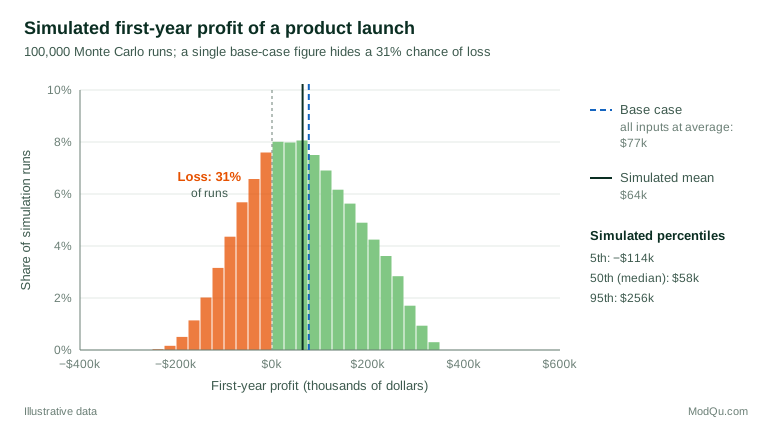
Why is the expected profit lower than the base case? Because of the capacity limit. When demand is high, sales are capped at 100,000 units, so the upside is cut off; when demand is low, the full shortfall hits profit. Whenever a model contains limits, thresholds or other non-linear steps, plugging average inputs into it does not give the average outcome. This effect, known informally as the "flaw of averages", is one of the most practical reasons to simulate.
Choosing input distributions
The output can be no better than the inputs. Good practice draws on evidence wherever possible:
- Survey estimates come with sampling uncertainty that can be expressed directly as a distribution. A purchase rate based on 400 concept-test respondents, as in the example, can be represented by a beta distribution centred on the observed rate. Survey intent also tends to overstate actual purchase, so many analysts apply a calibration factor with its own uncertainty.
- Historical data, such as past launch results or cost records, can be used to fit distributions or be resampled directly.
- Expert judgement is often summarised with triangular or PERT distributions using a minimum, most likely and maximum value. Experts tend to give ranges that are too narrow, so it helps to ask explicitly for extreme scenarios (Morgan & Henrion, 1990).
- Bayesian posterior distributions are natural inputs, because they already express what is known about a parameter after seeing data. Markov chain Monte Carlo, which grew out of the algorithm of Metropolis et al. (1953), is itself a Monte Carlo method for drawing from such distributions (Gelman et al., 2013).
Do not forget correlation
Inputs are rarely independent. Market size and purchase rate may both be high in a strong economy; raw material and shipping costs often rise together. Ignoring positive correlation between inputs usually understates the spread of outcomes. Iman and Conover (1982) proposed a widely used method that imposes a chosen rank correlation on sampled inputs while preserving each input's own distribution.
How many runs are enough?
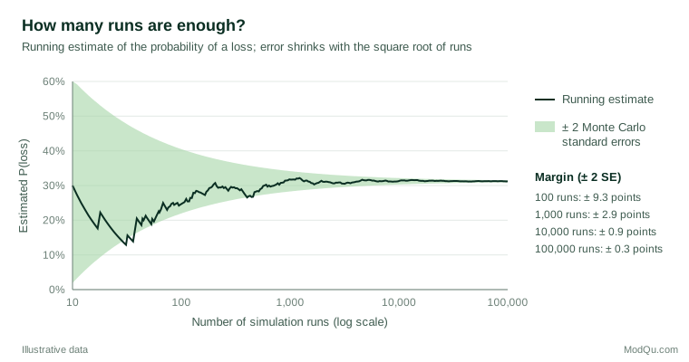
Monte Carlo results contain their own random error, which shrinks with the square root of the number of runs. For an estimated probability p from N runs, the Monte Carlo standard error is:
SE = √[ p(1 − p) ÷ N ]
In the launch example, 1,000 runs estimate the probability of loss to within about ±3 percentage points, while 100,000 runs bring that to about ±0.3 points (Figure 2). Ten times the precision needs one hundred times the runs. Tail probabilities, such as a 1-in-100 worst case, need far more runs than central estimates.
Two techniques improve efficiency. Latin hypercube sampling spreads draws evenly across each input's range rather than leaving it to chance, and often gives more precise results for the same number of runs (McKay et al., 1979). Variance reduction methods, such as antithetic and control variates, are standard in financial applications (Glasserman, 2003). Simulations also depend on good pseudo-random number generators; modern software uses well-tested algorithms such as the Mersenne Twister (Matsumoto & Nishimura, 1998). Fix and record the random seed so that results can be reproduced.
Uses in business and research
- Investment and launch decisions: probability of loss, payback period and value at risk for a project or product.
- Financial pricing: Boyle (1977) showed how simulation can value options, and it is now routine for complex derivatives (Glasserman, 2003).
- Project schedules and budgets: the chance of finishing on time when many tasks have uncertain durations.
- Measurement uncertainty: international metrology guidance sets out Monte Carlo propagation of distributions as an alternative to approximate formulas (Joint Committee for Guides in Metrology [JCGM], 2008).
- Survey design and analysis: simulating fieldwork outcomes to plan sample sizes, or testing how a weighting or modelling method performs when the truth is known.
Sensitivity analysis: which inputs matter?
A simulation also shows where uncertainty comes from. Simple approaches rank inputs by their correlation with the outcome and display the result as a tornado chart; variance-based methods divide the output variance among inputs and their interactions (Saltelli et al., 2008). In the launch example, squared rank correlations show that the purchase rate accounts for roughly half of the variation in profit and unit cost for about a third, which suggests that a larger concept test or an in-market trial would reduce risk more than refining cost estimates.
Common mistakes
- False precision. Reporting "a 31.22% chance of loss" implies more certainty than the input assumptions support. Round results and state the main assumptions.
- Ranges that are too narrow. Overconfident inputs produce overconfident outputs.
- Ignoring correlation between inputs that move together.
- Confusing model risk with input risk. Simulation only explores uncertainty within the model. If the model omits a competitor response or a supply failure, so does the simulation.
- Presenting only the mean. The value of the method lies in the distribution. Spiegelhalter et al. (2011) show that fan charts, histograms and plain statements of chance help audiences understand uncertainty.
Key takeaways
Monte Carlo simulation replaces a single fragile forecast with a distribution of plausible outcomes. It exposes the chance of loss, corrects the "flaw of averages" in non-linear models and shows which inputs drive risk. Its value depends on evidence-based input distributions, realistic correlations, enough runs for the precision needed and honest communication of what the model leaves out.
References
Boyle, P. P. (1977). Options: A Monte Carlo approach. Journal of Financial Economics, 4(3), 323–338. https://doi.org/10.1016/0304-405X(77)90005-8
Gelman, A., Carlin, J. B., Stern, H. S., Dunson, D. B., Vehtari, A., & Rubin, D. B. (2013). Bayesian data analysis (3rd ed.). Chapman and Hall/CRC. https://doi.org/10.1201/b16018
Glasserman, P. (2003). Monte Carlo methods in financial engineering. Springer. https://doi.org/10.1007/978-0-387-21617-1
Iman, R. L., & Conover, W. J. (1982). A distribution-free approach to inducing rank correlation among input variables. Communications in Statistics - Simulation and Computation, 11(3), 311–334. https://doi.org/10.1080/03610918208812265
Joint Committee for Guides in Metrology. (2008). Evaluation of measurement data: Supplement 1 to the "Guide to the expression of uncertainty in measurement": Propagation of distributions using a Monte Carlo method (JCGM 101:2008). Bureau International des Poids et Mesures.
Kroese, D. P., Taimre, T., & Botev, Z. I. (2011). Handbook of Monte Carlo methods. Wiley. https://doi.org/10.1002/9781118014967
Matsumoto, M., & Nishimura, T. (1998). Mersenne twister: A 623-dimensionally equidistributed uniform pseudo-random number generator. ACM Transactions on Modeling and Computer Simulation, 8(1), 3–30. https://doi.org/10.1145/272991.272995
McKay, M. D., Beckman, R. J., & Conover, W. J. (1979). Comparison of three methods for selecting values of input variables in the analysis of output from a computer code. Technometrics, 21(2), 239–245. https://doi.org/10.1080/00401706.1979.10489755
Metropolis, N., Rosenbluth, A. W., Rosenbluth, M. N., Teller, A. H., & Teller, E. (1953). Equation of state calculations by fast computing machines. The Journal of Chemical Physics, 21(6), 1087–1092. https://doi.org/10.1063/1.1699114
Metropolis, N., & Ulam, S. (1949). The Monte Carlo method. Journal of the American Statistical Association, 44(247), 335–341. https://doi.org/10.1080/01621459.1949.10483310
Morgan, M. G., & Henrion, M. (1990). Uncertainty: A guide to dealing with uncertainty in quantitative risk and policy analysis. Cambridge University Press. https://doi.org/10.1017/CBO9780511840609
Robert, C. P., & Casella, G. (2004). Monte Carlo statistical methods (2nd ed.). Springer. https://doi.org/10.1007/978-1-4757-4145-2
Saltelli, A., Ratto, M., Andres, T., Campolongo, F., Cariboni, J., Gatelli, D., Saisana, M., & Tarantola, S. (2008). Global sensitivity analysis: The primer. Wiley. https://doi.org/10.1002/9780470725184
Spiegelhalter, D., Pearson, M., & Short, I. (2011). Visualizing uncertainty about the future. Science, 333(6048), 1393–1400. https://doi.org/10.1126/science.1191181