
Statistics · Bayesian and computational
Bayesian Inference in Market Research
How Bayesian inference combines prior knowledge with new survey data, why it suits small samples and concept tests, and how to choose priors and report results honestly.
Market researchers rarely start from nothing. A brand team testing its tenth snack concept knows roughly how earlier concepts performed; a tracking study has years of previous waves. Bayesian inference is a formal way of combining that existing knowledge with new data. It treats an unknown quantity, such as the share of buyers who would try a product, as uncertain, describes that uncertainty with a probability distribution, and updates it as evidence arrives. The idea goes back to Bayes (1763), and modern computing has made it a practical everyday tool (Gelman et al., 2013).
How the updating works
Bayes' theorem links three pieces:
posterior ∝ likelihood × prior
The prior expresses what is believed before the new data are seen. The likelihood describes how probable the observed data are for each possible value of the quantity. The posterior is the updated belief, and everything reported comes from it: a best estimate, a 95% credible interval, and direct probability statements such as "there is a 74% chance that more than half of the target market would buy".
That last kind of statement is the main practical attraction. A frequentist confidence interval is often misread as saying exactly this, but only a Bayesian analysis can say it legitimately (Kruschke & Liddell, 2018).
A worked example: a concept test
Suppose, hypothetically, that 36 of 60 respondents in a concept test say they would definitely or probably buy a new product, a raw rate of 60%. Across the company's past concepts, intent has averaged about 40%, and the team summarises this history as a Beta(12, 18) prior distribution, which carries roughly as much information as 30 earlier respondents.
With a beta prior and yes/no answers, the posterior is also a beta distribution: add the "yes" answers to the first number and the "no" answers to the second. The result is Beta(12 + 36, 18 + 24) = Beta(48, 42).
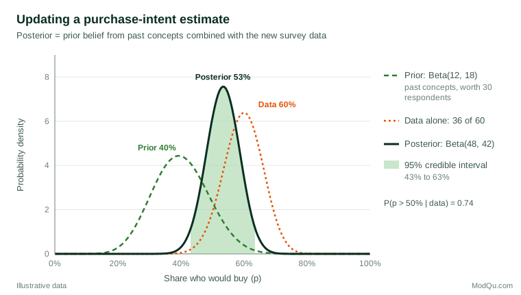
The posterior mean is 53%, with a 95% credible interval of 43% to 63%, and a 74% probability that true intent exceeds 50%. Using the data alone, with a flat prior, the estimate would be about 60% and that probability about 94%. The prior pulls an unusually good small-sample result back towards the historical norm. This "shrinkage" protects against over-reacting to noise, which is exactly what a sensible manager would do informally.
Where Bayesian methods help in market research
- Small samples and many subgroups. Hierarchical models let estimates for small regions or segments borrow strength from the whole sample. Wang et al. (2015) used this approach, with poststratification, to produce accurate election forecasts from a heavily unrepresentative online panel.
- Choice modelling and conjoint. Hierarchical Bayes estimation of individual-level preferences is now standard in conjoint analysis, and Rossi and Allenby (2003) review its wide use in marketing.
- Sequential and tracking studies. Each wave's posterior can serve as the next wave's prior, giving smoother trend lines without discarding history.
- Decisions. Posterior probabilities feed directly into expected-value calculations, such as the chance a launch clears a revenue hurdle.
Choosing and checking priors
Priors are the most debated part of the method. Good practice is to base them on documented evidence, such as past studies, norms or expert judgement, and to state them openly. Gelman, Simpson and Betancourt (2017) stress that a prior can only be judged alongside the likelihood and the data it will meet: a prior that looks harmless may dominate a small sample. Prior predictive checks, which simulate data the prior implies, reveal priors that allow absurd results.
Common mistakes
- Hiding the prior. Readers cannot judge a result if they do not know what was assumed. Report the prior and its source.
- Skipping sensitivity analysis. Re-run the analysis with a weaker and a stronger prior. If conclusions change materially, say so.
- Treating "Bayesian" as a cure for bad data. A prior does not fix a biased sample or a leading question.
- Ignoring convergence. Complex models are fitted by simulation (Markov chain Monte Carlo), and the chains must be checked before the results are trusted (McElreath, 2020).
Key takeaways
Bayesian inference turns prior knowledge and new evidence into a single, interpretable statement of uncertainty. For concept tests, small segments and repeated tracking it often gives steadier and more decision-friendly results than treating each study in isolation. Its value depends on transparent, defensible priors and on showing how much they matter.
References
Bayes, T. (1763). An essay towards solving a problem in the doctrine of chances. Philosophical Transactions of the Royal Society of London, 53, 370–418. https://doi.org/10.1098/rstl.1763.0053
Gelman, A., Carlin, J. B., Stern, H. S., Dunson, D. B., Vehtari, A., & Rubin, D. B. (2013). Bayesian data analysis (3rd ed.). Chapman and Hall/CRC. https://doi.org/10.1201/b16018
Gelman, A., Simpson, D., & Betancourt, M. (2017). The prior can often only be understood in the context of the likelihood. Entropy, 19(10), Article 555. https://doi.org/10.3390/e19100555
Kruschke, J. K., & Liddell, T. M. (2018). The Bayesian New Statistics: Hypothesis testing, estimation, meta-analysis, and power analysis from a Bayesian perspective. Psychonomic Bulletin & Review, 25(1), 178–206. https://doi.org/10.3758/s13423-016-1221-4
McElreath, R. (2020). Statistical rethinking: A Bayesian course with examples in R and Stan (2nd ed.). Chapman and Hall/CRC. https://doi.org/10.1201/9780429029608
Rossi, P. E., & Allenby, G. M. (2003). Bayesian statistics and marketing. Marketing Science, 22(3), 304–328. https://doi.org/10.1287/mksc.22.3.304.17739
Wang, W., Rothschild, D., Goel, S., & Gelman, A. (2015). Forecasting elections with non-representative polls. International Journal of Forecasting, 31(3), 980–991. https://doi.org/10.1016/j.ijforecast.2014.06.001