
Statistics · Bayesian and computational
Multilevel Regression and Post-Stratification (MRP)
How MRP turns a national or unrepresentative survey into reliable estimates for provinces, regions and small segments, with a worked example, practical guidance and the mistakes to avoid.
Clients often want answers for groups that a survey was never designed to measure. A national study of 1,500 adults may be asked to report purchase intent in each province, in each age band within each region, or among owners of a particular car brand. Splitting the sample leaves some cells with a handful of respondents, and the resulting percentages jump from wave to wave for no real reason. Many online samples also over-represent young, educated or highly engaged people.
Multilevel regression and post-stratification (MRP, sometimes nicknamed "Mister P") tackles both problems at once. It fits a regression model that predicts the outcome for every combination of demographic and geographic characteristics, then reweights those predictions to the known make-up of the population. The method was introduced for estimating opinion in American states from national polls (Gelman & Little, 1997; Park et al., 2004) and is now used in political science, public health and commercial research.
The problem MRP solves
There are two traditional ways to estimate a quantity for a small area. Disaggregation simply takes the respondents who live there and computes their average. It is unbiased only if the subsample is representative, and it is very noisy when the subsample is small. Weighting adjusts the sample so that its totals match known population totals, for example by raking to age, sex and region (Deville & Särndal, 1992; Valliant et al., 2018). Weighting corrects some imbalance, but it can only use a few variables before the weights become extreme, and it does nothing to stabilise estimates for small areas.
MRP borrows ideas from both small area estimation and model-based survey inference. Instead of treating each area separately, it lets areas and demographic groups share information through a model, and it uses population data to say how many people of each type live in each area (Rao & Molina, 2015; Little, 1993).
The two steps
Step 1: multilevel regression
The analyst divides the population into poststratification cells, defined by every combination of the variables in the model, such as province × age band × sex × education. A multilevel model, usually a logistic regression for a yes/no outcome, then predicts the outcome in each cell. For respondent i:
logit Pr(yi = 1) = β0 + αagea[i] + αsexs[i] + αedue[i] + αprovp[i] + γ zp[i]
Each set of α terms is a random effect, given a normal distribution with its own standard deviation that the data estimate. A province with few respondents has its effect pulled towards zero, so its prediction leans on the national pattern and on the province-level predictor z. Province-level predictors, such as past market share, average income or category penetration, matter a great deal: they tell the model why provinces differ, and they let it make good predictions for provinces with little data (Gelman & Hill, 2007; Buttice & Highton, 2013).
Step 2: post-stratification
The model gives a predicted probability θ̂c for every cell c, including cells with no respondents at all. These predictions are then averaged with the population count Nc of each cell as the weight. For province p:
θ̂p = Σc ∈ p Nc θ̂c ÷ Σc ∈ p Nc
The cell counts come from a census, a large official survey or a high-quality register. Because the final estimate depends on the population mix rather than the sample mix, an over-representation of young graduates in the sample no longer distorts the result, provided the model captures how the outcome varies with age and education.
A worked example
To show how the method behaves when the truth is known, we built a hypothetical population in which the share of adults intending to switch their home internet provider in the next year varies by province, age, sex and education. Provinces were given their approximate relative sizes. We then drew an online-style sample of 1,500 people in which young adults and degree holders were over-represented: 54% of the sample was aged 18 to 34, against 27% of the population, and 57% held a degree, against about 39%.
In the simulated population, 36.8% of adults intended to switch. The raw sample said 48.7%, because the over-represented groups were more likely to switch. The province estimates were worse. Prince Edward Island had only 7 respondents, and New Brunswick 34; their raw percentages were 43% and 56%, against true values of 29% and 28%.
We fitted the model above, with a province-level predictor for category penetration, and post-stratified to the population cells. The MRP national estimate was 37.9%. Across the ten provinces, the average absolute error fell from 12.6 percentage points for the raw subsample percentages to 2.4 points for MRP.
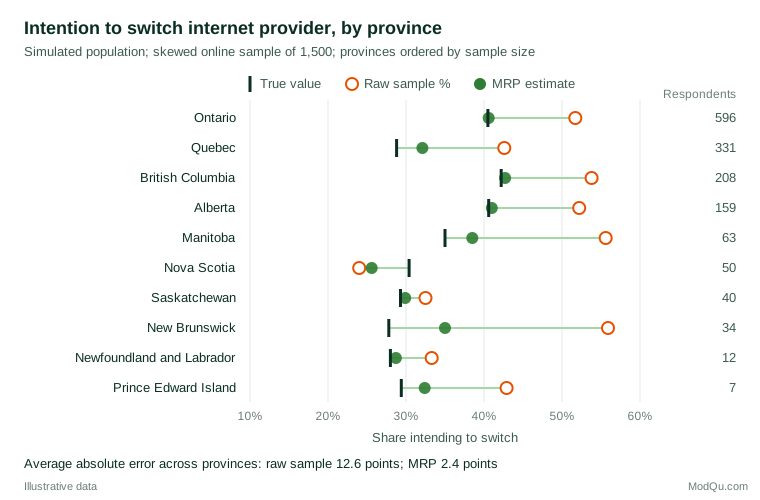
The result has two lessons. First, MRP was not perfect. It put New Brunswick at 35.0% against a true 27.8%, and Nova Scotia at 25.6% against 30.4%. With few respondents, these estimates lean heavily on the model and on the province-level predictor, and whatever makes a province distinctive beyond those inputs is partly lost. Models make assumptions, and when those assumptions miss, the estimates inherit the error. Second, most of the improvement in the large provinces came from post-stratification, which corrected the age and education skew, while most of the improvement in the small provinces came from partial pooling, which stopped seven interviews from being treated as a reliable measurement.
Why MRP works, and when it does not
The best-known demonstration is the study by Wang et al. (2015), who collected opinion polls through an online gaming platform whose users were overwhelmingly young and male. Raw results were badly wrong, but after MRP with detailed demographic cells and previous vote, the forecasts were close to those of established polling averages. Lax and Phillips (2009) found that MRP estimates of state opinion from a single national survey compared well with disaggregation of many pooled surveys. In public health, Zhang et al. (2014) used MRP with a national health survey to estimate disease prevalence for counties, and Downes et al. (2018) argue that it can reduce selection bias in highly selected study samples.
These successes depend on conditions that are worth stating plainly:
- The model must contain the variables that drive both selection and the outcome. MRP adjusts only for what is in the cells. If heavy internet users are more likely both to join a panel and to switch provider, and internet use is not in the model, the bias remains. This is the same requirement that governs every adjustment of a nonprobability sample (Elliott & Valliant, 2017).
- Group-level predictors carry much of the weight. Buttice and Highton (2013) found that MRP performed well for some opinions and poorly for others, and that performance depended strongly on how well the area-level predictors explained differences between areas.
- The population frame must be accurate. Cell counts that are out of date or measured differently from the survey variables introduce their own error. If the survey asks about education in different categories from the census, the categories must be harmonised.
- Interactions may be needed. If young people in Quebec behave differently from young people elsewhere, a model with only main effects will miss it. Ghitza and Gelman (2013) show how deep interactions between geography and demographics can be estimated with multilevel priors, and Gao et al. (2021) show that structured priors for ordered categories such as age can improve small-group estimates.
MRP and weighting compared
Weighting and MRP rest on the same idea: the sample must be made to look like the population on the variables that matter. Weighting does this by changing how much each respondent counts, MRP by modelling the outcome and projecting it onto the population. Gelman (2007) argues that regression modelling and weighting are best seen as two routes to the same goal, and that the modelling route handles many adjustment variables and small domains more gracefully.
| Weighting (raking or calibration) | MRP | |
|---|---|---|
| Adjustment variables | A few, before weights become extreme | Many, including interactions |
| Small areas | Noisy, often unusable | Stabilised by partial pooling |
| Estimates for several outcomes | One set of weights for all | A model for each outcome |
| Transparency | Easy to explain and audit | Requires model checking and documentation |
| Population data needed | Marginal totals | Joint cell counts |
In practice the two are complementary. Many organisations publish weighted national figures and use MRP for regional or segment breakdowns. Model-based approaches have also been central to the debate about polling errors: an evaluation of the 2016 United States election polls found that failure to adjust for education was one reason many state polls were wrong (Kennedy et al., 2018), a problem that cell-based adjustment such as MRP is designed to address when education is in the model.
Practical guidance for survey and business research
- Start from the reporting groups. Include every area or segment to be reported as a grouping factor, and check that population counts exist for it.
- Use the best available frame. Census tables are the usual source; for customer populations, a customer database with reliable demographics can serve as the frame.
- Invest in area-level predictors. Past sales, market share, store density or regional income often explain more variation between areas than the survey data alone can.
- Fit the model with modern software. Bayesian fitting with Stan, a widely used probabilistic programming language, propagates uncertainty from the model into every cell and every aggregate (Carpenter et al., 2017).
- Report uncertainty. Give intervals for every estimate; small areas keep wider intervals even after pooling.
- Validate where you can. Compare MRP estimates for large areas with direct estimates, and compare against external benchmarks such as sales data or official statistics.
Common mistakes
- Treating MRP as a cure for any sample. It cannot correct for selection on variables that are not in the model.
- Omitting area-level predictors. Without them, small areas are simply pulled towards the national average, which can hide real regional differences.
- Using a mismatched frame. Survey categories and population categories must be defined the same way.
- Reporting estimates for areas with no data as if they were measurements. Estimates for cells or areas with few respondents rest mainly on the model and should be labelled as modelled.
- Skipping model checks. Compare predictions with observed data in held-out groups, and examine whether residual differences between areas remain (Lohr, 2021).
Key takeaways
MRP combines a multilevel regression model with population counts to produce estimates for areas and segments that a survey alone cannot support. It corrects demographic imbalance through post-stratification and stabilises small groups through partial pooling. It works best when the model includes the variables that drive both selection and the outcome, when strong area-level predictors are available and when the population frame is accurate. Used with honest uncertainty and external validation, it turns national and even unrepresentative samples into credible regional evidence.
References
Buttice, M. K., & Highton, B. (2013). How does multilevel regression and poststratification perform with conventional national surveys? Political Analysis, 21(4), 449–467. https://doi.org/10.1093/pan/mpt017
Carpenter, B., Gelman, A., Hoffman, M. D., Lee, D., Goodrich, B., Betancourt, M., Brubaker, M., Guo, J., Li, P., & Riddell, A. (2017). Stan: A probabilistic programming language. Journal of Statistical Software, 76(1), 1–32. https://doi.org/10.18637/jss.v076.i01
Deville, J.-C., & Särndal, C.-E. (1992). Calibration estimators in survey sampling. Journal of the American Statistical Association, 87(418), 376–382. https://doi.org/10.1080/01621459.1992.10475217
Downes, M., Gurrin, L. C., English, D. R., Pirkis, J., Currier, D., Spittal, M. J., & Carlin, J. B. (2018). Multilevel regression and poststratification: A modeling approach to estimating population quantities from highly selected survey samples. American Journal of Epidemiology, 187(8), 1780–1790. https://doi.org/10.1093/aje/kwy070
Elliott, M. R., & Valliant, R. (2017). Inference for nonprobability samples. Statistical Science, 32(2), 249–264. https://doi.org/10.1214/16-STS598
Gao, Y., Kennedy, L., Simpson, D., & Gelman, A. (2021). Improving multilevel regression and poststratification with structured priors. Bayesian Analysis, 16(3), 719–744. https://doi.org/10.1214/20-BA1223
Gelman, A. (2007). Struggles with survey weighting and regression modeling. Statistical Science, 22(2), 153–164. https://doi.org/10.1214/088342306000000691
Gelman, A., & Hill, J. (2007). Data analysis using regression and multilevel/hierarchical models. Cambridge University Press. https://doi.org/10.1017/CBO9780511790942
Gelman, A., & Little, T. C. (1997). Poststratification into many categories using hierarchical logistic regression. Survey Methodology, 23(2), 127–135.
Ghitza, Y., & Gelman, A. (2013). Deep interactions with MRP: Election turnout and voting patterns among small electoral subgroups. American Journal of Political Science, 57(3), 762–776. https://doi.org/10.1111/ajps.12004
Kennedy, C., Blumenthal, M., Clement, S., Clinton, J. D., Durand, C., Franklin, C., McGeeney, K., Miringoff, L., Olson, K., Rivers, D., Saad, L., Witt, G. E., & Wlezien, C. (2018). An evaluation of the 2016 election polls in the United States. Public Opinion Quarterly, 82(1), 1–33. https://doi.org/10.1093/poq/nfx047
Lax, J. R., & Phillips, J. H. (2009). How should we estimate public opinion in the states? American Journal of Political Science, 53(1), 107–121. https://doi.org/10.1111/j.1540-5907.2008.00360.x
Little, R. J. A. (1993). Post-stratification: A modeler's perspective. Journal of the American Statistical Association, 88(423), 1001–1012. https://doi.org/10.1080/01621459.1993.10476368
Lohr, S. L. (2021). Sampling: Design and analysis (3rd ed.). Chapman and Hall/CRC. https://doi.org/10.1201/9780429298899
Park, D. K., Gelman, A., & Bafumi, J. (2004). Bayesian multilevel estimation with poststratification: State-level estimates from national polls. Political Analysis, 12(4), 375–385. https://doi.org/10.1093/pan/mph024
Rao, J. N. K., & Molina, I. (2015). Small area estimation (2nd ed.). Wiley. https://doi.org/10.1002/9781118735855
Valliant, R., Dever, J. A., & Kreuter, F. (2018). Practical tools for designing and weighting survey samples (2nd ed.). Springer. https://doi.org/10.1007/978-3-319-93632-1
Wang, W., Rothschild, D., Goel, S., & Gelman, A. (2015). Forecasting elections with non-representative polls. International Journal of Forecasting, 31(3), 980–991. https://doi.org/10.1016/j.ijforecast.2014.06.001
Zhang, X., Holt, J. B., Lu, H., Wheaton, A. G., Ford, E. S., Greenlund, K. J., & Croft, J. B. (2014). Multilevel regression and poststratification for small-area estimation of population health outcomes: A case study of chronic obstructive pulmonary disease prevalence using the Behavioral Risk Factor Surveillance System. American Journal of Epidemiology, 179(8), 1025–1033. https://doi.org/10.1093/aje/kwu018