
Statistics · Bayesian and computational
Simulation Studies for Evaluating Statistical Method Performance
How simulation studies test statistical methods on data where the truth is known, which performance measures to use, how many repetitions are enough and how to report results honestly.
Every statistical method rests on assumptions, and real data rarely satisfy them exactly. Survey responses are skewed, groups have unequal sizes and spreads, samples are weighted and some cells are tiny. Will a confidence interval still cover the true value 95% of the time? Will a test still produce false alarms only 5% of the time? Mathematical theory often answers these questions only for very large samples or idealised conditions.
A simulation study answers them empirically. The analyst invents a world in which the truth is known, generates many data sets from it, applies the method to each one and records how often and by how much the method gets the answer right. Because the truth is set by the analyst, the method's errors can be measured directly, something that is impossible with real data. Simulation is now one of the main tools of methodological research and an increasingly common part of applied analysis planning (Morris et al., 2019; Boulesteix et al., 2020).
From Monte Carlo to method evaluation
Simulation studies are a form of Monte Carlo simulation, a family of methods that use repeated random sampling to approximate quantities that are hard to compute exactly. The name and the systematic approach date from work at Los Alamos in the 1940s (Metropolis & Ulam, 1949), and modern computing has made Monte Carlo methods a routine part of statistics (Robert & Casella, 2004). They differ from the bootstrap (Efron, 1979), which resamples the observed data to estimate uncertainty in one analysis; a simulation study draws from a model chosen by the analyst to evaluate a method in general.
Many familiar rules of thumb come from simulation studies. The guideline of at least 10 events per predictor in logistic regression came from simulations by Peduzzi et al. (1996), and later simulations by Vittinghoff and McCulloch (2007) suggested that it can often be relaxed. Advice on the number of groups needed in multilevel models comes from simulations such as those of Maas and Hox (2005). The finding that t-tests and linear regression remain valid for large samples of very skewed data, such as health costs, was also demonstrated by simulation (Lumley et al., 2002).
Planning a simulation study
Morris et al. (2019) organise the planning of a simulation study around five elements, summarised by the acronym ADEMP:
- Aims. What question is the study meant to answer? For example: does a test control false alarms when group variances differ?
- Data-generating mechanisms. The models used to create data sets, varied across realistic scenarios: sample sizes, effect sizes, degrees of skewness, amounts of missing data.
- Estimands. The true quantities the methods try to estimate, such as a difference in means or a population proportion.
- Methods. The competing analyses applied to every simulated data set.
- Performance measures. The criteria used to judge the methods.
Burton et al. (2006) give a similar checklist and stress that every element should be written down in a protocol before any code is run.
Measuring performance
If θ is the true value and θ̂i is the estimate from simulated data set i out of nsim, the most common performance measures are:
Bias = (1 ÷ nsim) Σ θ̂i − θ
- Empirical standard error: the standard deviation of the θ̂i across repetitions, showing how much the estimate varies from sample to sample.
- Mean squared error: the average of (θ̂i − θ)², combining bias and variability.
- Coverage: the share of confidence intervals that contain θ. A nominal 95% interval should cover about 95% of the time.
- Type I error rate: when the true effect is zero, the share of tests that reject the null hypothesis. It should be close to the nominal level, usually 5%.
- Power: when a real effect exists, the share of tests that detect it.
Each of these is itself an estimate based on a finite number of repetitions, so it has its own uncertainty, the Monte Carlo standard error (Koehler et al., 2009). For a rejection rate or coverage proportion p:
MCSE = √(p (1 − p) ÷ nsim)
Rearranging gives the number of repetitions needed for a chosen precision: nsim = p (1 − p) ÷ MCSE². To estimate a 5% error rate to within about ±0.44 percentage points (two Monte Carlo standard errors of 0.22), 10,000 repetitions are needed. A study reporting a Type I error of 6% from 200 repetitions cannot distinguish it from 5%.
A worked example: comparing two t-tests
A retailer is piloting a new store layout and wants to compare mean basket spend between pilot stores and control stores. The analyst must choose between Student's t-test, which assumes the two groups have equal variances, and Welch's t-test, which does not. Delacre et al. (2017) argue that Welch's test should be the default. A small simulation shows why.
We generated data for four hypothetical scenarios, each with the same true mean of $50 in both groups, so that every rejection is a false alarm. We ran 10,000 repetitions per scenario, applied both tests at the 5% level and recorded the rejection rates.
| Scenario | Pilot group (n, SD) | Control group (n, SD) | Student's t | Welch's t |
|---|---|---|---|---|
| Equal sizes, equal spread | 40, $10 | 40, $10 | 5.09% | 5.09% |
| Equal sizes, unequal spread | 40, $20 | 40, $10 | 5.05% | 4.95% |
| Small group more variable | 20, $20 | 80, $10 | 18.66% | 5.32% |
| Large group more variable | 80, $20 | 20, $10 | 0.44% | 4.67% |
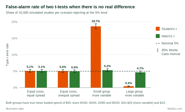
With equal group sizes, the two tests behave almost identically, even when spreads differ. When a small, variable pilot group is compared with a large, stable control group, Student's test raises a false alarm almost one time in five. In the reverse case it almost never rejects, which means it would also miss real effects. Welch's test stays within Bradley's (1978) widely used "liberal" criterion of 2.5% to 7.5% in every scenario. The Monte Carlo standard error is about 0.22 percentage points for rates near 5%, so the differences between the tests are far larger than simulation noise.
A natural extension is to add scenarios with a real difference, say $5 in mean spend, and record power. Error rates alone are not enough: a test that never rejects has a perfect false-alarm rate and is useless. Good method comparisons always report error control and power together.
The business lesson is direct. Pilot programmes often involve a few stores, regions or customers with unusual variability compared with a large control group, which is exactly the situation in which the default choice matters.
Uses in business and survey research
Simulation is not only for methodologists. Applied analysts use it to:
- Plan sample sizes for complex designs. When no formula exists, for example for clustered samples, weighted analyses or multilevel models, power can be estimated by simulating the planned design many times and counting how often the effect is detected (Arnold et al., 2011).
- Check an analysis plan before fieldwork. Simulating plausible data and running the planned analysis reveals problems such as empty cells, unstable weights or models that fail to converge.
- Compare estimators for a specific problem. Before choosing between weighting and model-based adjustment for a panel, an analyst can simulate data with realistic selection patterns and see which approach recovers the truth.
- Explain uncertainty to stakeholders. Showing how much a key figure varies across simulated repeat surveys is often more persuasive than quoting a standard error.
Good practice
- Use realistic scenarios. Base data-generating mechanisms on real data: observed sample sizes, skewness, correlations and missing-data patterns. Methods that win in unrealistic scenarios may lose in practice.
- Vary one factor at a time, and then in combination. The t-test example shows that unequal spread alone did little harm; the combination of unequal spread and unequal size did the damage.
- Keep the design manageable. Full factorial designs grow quickly: four sample sizes, three effect sizes and three variance ratios already give 36 scenarios. Choose factor levels that span the conditions met in practice, and spend repetitions where the methods are expected to differ.
- Run enough repetitions and report Monte Carlo standard errors for every performance measure (Koehler et al., 2009; Morris et al., 2019).
- Make the study reproducible. Set and report random-number seeds, record software versions and share code. Modern generators such as the Mersenne Twister produce very long, well-tested pseudo-random sequences (Matsumoto & Nishimura, 1998).
- Report the computational details. Hoaglin and Andrews (1975) argued long ago that results based on computation should be reported with enough detail to be checked and repeated, and the point still applies.
- Handle failures openly. If a method fails to converge in some repetitions, report how often and how those repetitions were treated.
Common mistakes and limitations
- Too few repetitions. Differences of one or two percentage points in coverage or error rates are meaningless if the Monte Carlo standard error is of the same size.
- Selective scenarios. A developer can make almost any method look best by choosing favourable conditions. Boulesteix et al. (2013) call for neutral comparison studies by authors with no stake in the methods compared, and the parallel with selective reporting in empirical research is close (Simmons et al., 2011).
- Confusing the simulated world with the real one. A simulation shows how a method performs when the data-generating model is true. If real data are generated differently, the conclusions may not transfer.
- Reporting only averages. Summaries such as average bias can hide scenarios in which a method fails badly. Present results by scenario, ideally in graphs.
- Ignoring the analysis pipeline. Real analyses include data cleaning, model selection and weighting steps. Simulating only the final test can overstate how well the whole process works.
Key takeaways
Simulation studies test statistical methods in worlds where the truth is known, which makes it possible to measure bias, precision, coverage, error rates and power directly. A good study states its aims, data-generating mechanisms, estimands, methods and performance measures in advance, uses realistic scenarios, runs enough repetitions and reports Monte Carlo standard errors. For business and survey analysts, small targeted simulations are a practical way to choose methods, plan sample sizes and check that an analysis will behave as intended before decisions depend on it.
References
Arnold, B. F., Hogan, D. R., Colford, J. M., Jr., & Hubbard, A. E. (2011). Simulation methods to estimate design power: An overview for applied research. BMC Medical Research Methodology, 11, Article 94. https://doi.org/10.1186/1471-2288-11-94
Boulesteix, A.-L., Groenwold, R. H. H., Abrahamowicz, M., Binder, H., Briel, M., Hornung, R., Morris, T. P., Rahnenführer, J., & Sauerbrei, W. (2020). Introduction to statistical simulations in health research. BMJ Open, 10(12), Article e039921. https://doi.org/10.1136/bmjopen-2020-039921
Boulesteix, A.-L., Lauer, S., & Eugster, M. J. A. (2013). A plea for neutral comparison studies in computational sciences. PLoS ONE, 8(4), Article e61562. https://doi.org/10.1371/journal.pone.0061562
Bradley, J. V. (1978). Robustness? British Journal of Mathematical and Statistical Psychology, 31(2), 144–152. https://doi.org/10.1111/j.2044-8317.1978.tb00581.x
Burton, A., Altman, D. G., Royston, P., & Holder, R. L. (2006). The design of simulation studies in medical statistics. Statistics in Medicine, 25(24), 4279–4292. https://doi.org/10.1002/sim.2673
Delacre, M., Lakens, D., & Leys, C. (2017). Why psychologists should by default use Welch's t-test instead of Student's t-test. International Review of Social Psychology, 30(1), 92–101. https://doi.org/10.5334/irsp.82
Efron, B. (1979). Bootstrap methods: Another look at the jackknife. The Annals of Statistics, 7(1), 1–26. https://doi.org/10.1214/aos/1176344552
Hoaglin, D. C., & Andrews, D. F. (1975). The reporting of computation-based results in statistics. The American Statistician, 29(3), 122–126. https://doi.org/10.1080/00031305.1975.10477393
Koehler, E., Brown, E., & Haneuse, S. J.-P. A. (2009). On the assessment of Monte Carlo error in simulation-based statistical analyses. The American Statistician, 63(2), 155–162. https://doi.org/10.1198/tast.2009.0030
Lumley, T., Diehr, P., Emerson, S., & Chen, L. (2002). The importance of the normality assumption in large public health data sets. Annual Review of Public Health, 23(1), 151–169. https://doi.org/10.1146/annurev.publhealth.23.100901.140546
Maas, C. J. M., & Hox, J. J. (2005). Sufficient sample sizes for multilevel modeling. Methodology, 1(3), 86–92. https://doi.org/10.1027/1614-2241.1.3.86
Matsumoto, M., & Nishimura, T. (1998). Mersenne twister: A 623-dimensionally equidistributed uniform pseudo-random number generator. ACM Transactions on Modeling and Computer Simulation, 8(1), 3–30. https://doi.org/10.1145/272991.272995
Metropolis, N., & Ulam, S. (1949). The Monte Carlo method. Journal of the American Statistical Association, 44(247), 335–341. https://doi.org/10.1080/01621459.1949.10483310
Morris, T. P., White, I. R., & Crowther, M. J. (2019). Using simulation studies to evaluate statistical methods. Statistics in Medicine, 38(11), 2074–2102. https://doi.org/10.1002/sim.8086
Peduzzi, P., Concato, J., Kemper, E., Holford, T. R., & Feinstein, A. R. (1996). A simulation study of the number of events per variable in logistic regression analysis. Journal of Clinical Epidemiology, 49(12), 1373–1379. https://doi.org/10.1016/S0895-4356(96)00236-3
Robert, C. P., & Casella, G. (2004). Monte Carlo statistical methods (2nd ed.). Springer. https://doi.org/10.1007/978-1-4757-4145-2
Simmons, J. P., Nelson, L. D., & Simonsohn, U. (2011). False-positive psychology: Undisclosed flexibility in data collection and analysis allows presenting anything as significant. Psychological Science, 22(11), 1359–1366. https://doi.org/10.1177/0956797611417632
Vittinghoff, E., & McCulloch, C. E. (2007). Relaxing the rule of ten events per variable in logistic and Cox regression. American Journal of Epidemiology, 165(6), 710–718. https://doi.org/10.1093/aje/kwk052