
Statistics · Bayesian and computational
Bayesian Hierarchical Models for Partial Pooling and Knowledge Stabilization
How Bayesian hierarchical models let many small estimates borrow strength from one another, why this stabilises rankings and trends, and how to fit, check and report them.
Business analysts rarely estimate one number at a time. They estimate conversion rates for dozens of advertising creatives, return rates for hundreds of products, satisfaction for every sales agent and purchase intent for every concept in a pipeline. Some of these units have plenty of data; many have very little. Estimated one at a time, the small units produce extreme values that look like discoveries and then vanish the following month. Decisions built on them, such as which creative to scale or which product to drop, are built on noise.
A Bayesian hierarchical model treats such a set of related quantities as members of a family. Each unit has its own value, but the values are assumed to come from a common distribution whose centre and spread are learned from all the units together. The result is partial pooling: each estimate is a compromise between the unit's own data and the family average, weighted by how much the unit's data can be trusted (Gelman et al., 2013). Estimates that stay sensible as new data arrive are the "stabilised knowledge" that the title refers to.
Three ways to estimate many related quantities
Suppose we want the conversion rate of each of J creatives.
- No pooling uses each creative's own rate, yj ÷ nj. It is unbiased for each unit but very noisy for small nj, and the most extreme values are usually the least reliable.
- Complete pooling gives every creative the overall rate. It is stable but assumes, implausibly, that the creatives do not differ.
- Partial pooling estimates how much the creatives really differ and shrinks each raw rate towards the overall rate by an amount that depends on its sample size and on that real variation (Gelman & Hill, 2007).
The third option is not a split-the-difference compromise chosen by taste. Under a wide range of conditions it gives estimates that are closer to the truth, on average across units, than either extreme.
Stein's paradox: why shrinkage wins
The idea has a striking history. Stein showed in the 1950s that, when three or more means are estimated together, the obvious estimator, each sample mean on its own, can be beaten on total squared error by an estimator that pulls all of them towards a common value. James and Stein (1961) gave the explicit form of such an estimator. Efron and Morris (1975, 1977) brought the result to a wide audience with baseball: using the batting averages of 18 major-league players after their first 45 times at bat in 1970, shrunken estimates predicted the players' averages for the rest of the season considerably better than the players' own early averages did.
The explanation is regression to the mean. A player, product or branch with an extreme early result is, more often than not, partly lucky or unlucky. Shrinkage anticipates that correction. Lindley and Smith (1972) placed the idea in a fully Bayesian framework for linear models, and Morris (1983) developed the closely related empirical Bayes approach, in which the family distribution is estimated from the data and then treated as known.
The model
For proportions, a convenient hierarchical model is:
yj ~ Binomial(nj, θj), θj ~ Beta(μκ, (1 − μ)κ)
Here θj is the true rate for unit j, μ is the average rate across the family, and κ is a concentration parameter: large κ means the units are similar, small κ means they differ a lot. In a fully Bayesian analysis μ and κ receive their own prior distributions and are estimated together with the θj. Given μ and κ, the posterior mean of each rate has a simple form:
E(θj | data) = (yj + μκ) ÷ (nj + κ) = wj × (yj ÷ nj) + (1 − wj) × μ, wj = nj ÷ (nj + κ)
The family distribution acts like κ extra observations at the average rate. A unit with nj much larger than κ keeps nearly its own rate; a unit with nj much smaller than κ moves most of the way to the average. For continuous outcomes the normal–normal model works the same way, with the weight depending on the ratio of between-unit variance to sampling variance. Rubin's (1981) analysis of coaching effects in eight schools is the classic teaching example.
A worked example: twelve advertising creatives
A hypothetical retailer tests 12 online advertising creatives. Traffic was allocated unevenly, so the number of visits per creative ranges from 40 to 1,500. Across all 4,385 visits there were 253 purchases, a pooled conversion rate of 5.8%. Creative A converted 6 of 40 visitors (15.0%) and looks like a clear winner. Creative B converted 1 of 55 (1.8%) and looks like a failure.
We fitted the beta–binomial model above with a uniform prior on μ and a weakly informative prior on log κ, computing the posterior exactly on a fine grid. The posterior mean of μ was 6.1%, and the median of κ was about 435, which implies that the creatives' true rates differ with a standard deviation of only about 1.1 percentage points. Most of the spread in the raw rates was sampling noise.
For Creative A, the weight on its own data is about 40 ÷ (40 + 435) ≈ 0.08, so the estimate moves most of the way to the average. Its posterior mean is 7.1%, with a 90% credible interval of 4.9% to 10.5%. Creative B rises to 5.5%. Creative L, with 1,500 visits and a raw rate of 5.6%, has a weight of about 0.78 and barely moves, to 5.7%.
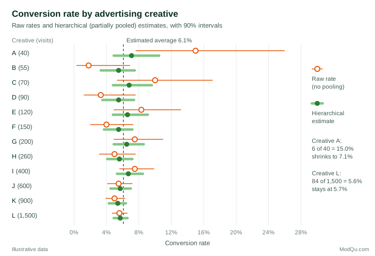
The practical consequences are large. On raw rates, A would be scaled up and B dropped. On posterior estimates, A is still the most promising creative, but its likely advantage is about one percentage point rather than nine, and there is substantial uncertainty about whether it beats the well-tested creatives at all. The sensible decision is to give A more traffic and learn more, not to reallocate the whole budget.
Why partial pooling stabilises knowledge
Rankings and league tables. Ranking units on raw rates systematically rewards small units with lucky samples. Goldstein and Spiegelhalter (1996) showed how wide the uncertainty in such rankings usually is, and Spiegelhalter (2005) proposed funnel plots that judge each unit against limits that widen as its sample shrinks. Hierarchical estimates address the same problem by building sample size into the estimate itself.
Many comparisons. When dozens of units are compared, some differences will look significant by chance. Gelman, Hill and Yajima (2012) argue that hierarchical models address this directly: because estimates are pulled together, spurious extreme differences shrink, and fewer false claims survive, without the blunt corrections used in classical multiple-comparison procedures.
Over time. Units that are re-estimated every month, such as store scores or agent ratings, swing less from wave to wave when they are partially pooled, because a single unusual month cannot drag the estimate far. Movements that do appear are more likely to be real.
New units. The fitted family distribution gives a sensible starting point for a unit that has not yet been tested. Before any data arrive, a new creative's best estimate is the family average, with an interval that reflects the real spread among creatives. As its own data accumulate, the estimate moves smoothly from that starting point towards its own rate, which suits test-and-learn programmes.
Individual-level marketing models. Hierarchical Bayes estimation of individual preferences in conjoint and choice studies applies the same logic to respondents: each person's few choices are combined with the distribution of preferences across the sample. Rossi and Allenby (2003) review how central this has become in marketing.
Fitting and checking hierarchical models
Simple models like the one above can be computed exactly, but most real models, with predictors, several grouping factors and non-normal outcomes, are fitted by Markov chain Monte Carlo (MCMC). Stan, a widely used probabilistic programming language, implements efficient Hamiltonian Monte Carlo for this purpose (Carpenter et al., 2017). Good practice includes:
- A sensible prior for the group-level spread. With few groups, the data say little about how much the groups differ, and the prior on that standard deviation matters. Gelman (2006) recommends weakly informative half-t or half-Cauchy priors rather than the once-common inverse-gamma priors with tiny parameters, which can distort results.
- A suitable parameterisation. When groups have little data, the sampler can struggle with the strong dependence between group effects and their spread. Writing the model in a non-centred form often solves this (Papaspiliopoulos et al., 2007).
- Convergence diagnostics. Run several chains and check that they agree. Vehtari et al. (2021) propose an improved R̂ statistic and recommend using samples only when it is below 1.01, together with adequate effective sample sizes.
- Predictive checks. Simulate data from the fitted model and compare them with the observed data, and simulate from the priors before fitting to see whether they allow absurd values. Gabry et al. (2019) show how plots of these checks fit into a Bayesian workflow.
A fully Bayesian analysis also carries uncertainty about μ and κ into every unit's interval. Empirical Bayes, which plugs in single estimates of these hyperparameters, is quicker and often gives similar point estimates, but its intervals tend to be too narrow when there are few groups (Morris, 1983; McElreath, 2020).
Limitations and common mistakes
- Pooling units that are not exchangeable. The model assumes that, before seeing the data, there is no reason to expect any particular unit to be higher or lower. If creatives differ systematically by format or channel, include those as predictors, so that each creative is pulled towards the average of comparable creatives rather than the grand average.
- Hiding genuine outliers. A truly exceptional unit with little data will be shrunk too. Shrinkage trades a small bias for a large reduction in noise; it does not make small samples informative. Collecting more data on promising units remains essential.
- Reading the posterior mean as a measurement. Report intervals and, where useful, the probability that a unit exceeds a business threshold.
- Too few groups. With only three or four units, the group-level spread is barely identified and the result depends heavily on its prior. Report a sensitivity analysis.
- Ignoring computational warnings. Divergent transitions and high R̂ values signal that the reported numbers may be wrong.
Key takeaways
Bayesian hierarchical models let many related estimates learn from one another. Each unit's estimate is pulled towards the family average by an amount that reflects its own sample size and the real variation among units, which makes rankings fairer, comparisons less prone to false alarms and trends steadier from wave to wave. The method rests on a sound theoretical basis, from Stein's paradox to modern Bayesian computation, and is now routine to fit. Its value in practice depends on including predictors that make units comparable, choosing sensible priors for the group-level spread, checking the computation and reporting uncertainty openly.
References
Carpenter, B., Gelman, A., Hoffman, M. D., Lee, D., Goodrich, B., Betancourt, M., Brubaker, M., Guo, J., Li, P., & Riddell, A. (2017). Stan: A probabilistic programming language. Journal of Statistical Software, 76(1), 1–32. https://doi.org/10.18637/jss.v076.i01
Efron, B., & Morris, C. (1975). Data analysis using Stein's estimator and its generalizations. Journal of the American Statistical Association, 70(350), 311–319. https://doi.org/10.1080/01621459.1975.10479864
Efron, B., & Morris, C. (1977). Stein's paradox in statistics. Scientific American, 236(5), 119–127. https://doi.org/10.1038/scientificamerican0577-119
Gabry, J., Simpson, D., Vehtari, A., Betancourt, M., & Gelman, A. (2019). Visualization in Bayesian workflow. Journal of the Royal Statistical Society Series A: Statistics in Society, 182(2), 389–402. https://doi.org/10.1111/rssa.12378
Gelman, A. (2006). Prior distributions for variance parameters in hierarchical models (Comment on article by Browne and Draper). Bayesian Analysis, 1(3), 515–533. https://doi.org/10.1214/06-BA117A
Gelman, A., Carlin, J. B., Stern, H. S., Dunson, D. B., Vehtari, A., & Rubin, D. B. (2013). Bayesian data analysis (3rd ed.). Chapman and Hall/CRC. https://doi.org/10.1201/b16018
Gelman, A., & Hill, J. (2007). Data analysis using regression and multilevel/hierarchical models. Cambridge University Press. https://doi.org/10.1017/CBO9780511790942
Gelman, A., Hill, J., & Yajima, M. (2012). Why we (usually) don't have to worry about multiple comparisons. Journal of Research on Educational Effectiveness, 5(2), 189–211. https://doi.org/10.1080/19345747.2011.618213
Goldstein, H., & Spiegelhalter, D. J. (1996). League tables and their limitations: Statistical issues in comparisons of institutional performance. Journal of the Royal Statistical Society Series A: Statistics in Society, 159(3), 385–443. https://doi.org/10.2307/2983325
James, W., & Stein, C. (1961). Estimation with quadratic loss. In J. Neyman (Ed.), Proceedings of the Fourth Berkeley Symposium on Mathematical Statistics and Probability (Vol. 1, pp. 361–379). University of California Press.
Lindley, D. V., & Smith, A. F. M. (1972). Bayes estimates for the linear model. Journal of the Royal Statistical Society Series B: Statistical Methodology, 34(1), 1–18. https://doi.org/10.1111/j.2517-6161.1972.tb00885.x
McElreath, R. (2020). Statistical rethinking: A Bayesian course with examples in R and Stan (2nd ed.). Chapman and Hall/CRC. https://doi.org/10.1201/9780429029608
Morris, C. N. (1983). Parametric empirical Bayes inference: Theory and applications. Journal of the American Statistical Association, 78(381), 47–55. https://doi.org/10.1080/01621459.1983.10477920
Papaspiliopoulos, O., Roberts, G. O., & Sköld, M. (2007). A general framework for the parametrization of hierarchical models. Statistical Science, 22(1), 59–73. https://doi.org/10.1214/088342307000000014
Rossi, P. E., & Allenby, G. M. (2003). Bayesian statistics and marketing. Marketing Science, 22(3), 304–328. https://doi.org/10.1287/mksc.22.3.304.17739
Rubin, D. B. (1981). Estimation in parallel randomized experiments. Journal of Educational Statistics, 6(4), 377–401. https://doi.org/10.3102/10769986006004377
Spiegelhalter, D. J. (2005). Funnel plots for comparing institutional performance. Statistics in Medicine, 24(8), 1185–1202. https://doi.org/10.1002/sim.1970
Vehtari, A., Gelman, A., Simpson, D., Carpenter, B., & Bürkner, P.-C. (2021). Rank-normalization, folding, and localization: An improved R̂ for assessing convergence of MCMC (with discussion). Bayesian Analysis, 16(2), 667–718. https://doi.org/10.1214/20-BA1221