
Statistics · Bayesian and computational
Bayesian Networks for Probabilistic Knowledge Representation
How Bayesian networks represent uncertain knowledge as a graph of variables and conditional probabilities, how they update beliefs when evidence arrives, and how to build and use them responsibly with survey and business data.
Business knowledge is rarely a single number. It is a web of relationships: service problems and price rises affect satisfaction, satisfaction affects survey scores and loyalty, and competitor activity affects loyalty too. Each link is uncertain. A Bayesian network is a way of writing such a web down precisely, so that it can be reasoned with. It combines a graph, which shows which variables directly influence which others, with probability tables, which say how strongly. Once built, the network answers questions such as "how likely is this customer to leave, given what we have just learned?" by applying Bayes' theorem consistently across every link.
Bayesian networks were developed in the 1980s as a way to reason under uncertainty in expert systems (Pearl, 1988), and they are now used in medicine, engineering, ecology, genetics, risk analysis and marketing (Koller & Friedman, 2009). This article explains how they work, walks through a small example, and sets out practical guidance and common pitfalls.
What a Bayesian network is
A Bayesian network has two parts.
- A directed acyclic graph. Each node is a variable, and each arrow points from a "parent" to a "child" that depends directly on it. "Acyclic" means that following the arrows never leads back to where you started.
- A conditional probability table for each node, giving the probability of each of its values for every combination of its parents' values. Nodes without parents simply have a prior probability.
Together these define a full joint probability distribution over all the variables. The key result is that the joint distribution factorises into local pieces, one per node:
P(X1, …, Xn) = Πi P(Xi | parents(Xi))
This factorisation is what makes Bayesian networks practical. A joint distribution over 20 yes/no variables would need more than a million probabilities if written out in full. A network in which each variable has at most three parents needs at most 160, because each table only involves a node and its parents.
The graph also encodes conditional independence. Each variable is independent of its non-descendants once its parents are known. More generally, a graphical criterion called d-separation reads off every independence that the graph implies (Pearl, 1988), and Lauritzen et al. (1990) proved that this criterion is equivalent to other formal statements of the network's independence properties. In practical terms, the graph is a compact, inspectable statement of which pieces of knowledge are relevant to which others.
A worked example: customer churn
Figure 1 shows a hypothetical network for a subscription business. A service problem and a price rise each make a customer more likely to be dissatisfied. Dissatisfaction makes a low score on a satisfaction survey more likely, and it also raises the chance of churn. A competitor offer independently raises the chance of churn.
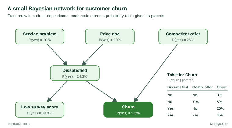
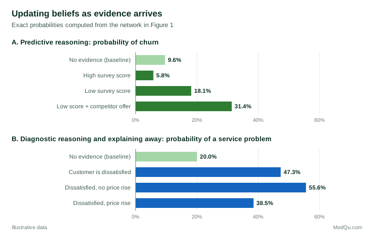
The whole model needs only 13 probabilities, against 63 for the full joint distribution of six yes/no variables. From these, the network computes that 24.3% of customers are dissatisfied, 30.8% give a low survey score, and 9.6% churn. The power of the network shows when evidence arrives (Figure 2).
Three kinds of reasoning appear in this hypothetical example.
- Predictive reasoning, from causes or signals towards outcomes. A low survey score almost doubles the estimated churn risk, from 9.6% to 18.1%. Adding the knowledge that the customer has received a competitor offer raises it to 31.4%. A high score lowers it to 5.8%.
- Diagnostic reasoning, from effects back to causes. Learning that a customer is dissatisfied raises the probability of an underlying service problem from 20% to 47.3%.
- Explaining away. If we also learn that the customer faced a price rise, the probability of a service problem falls to 38.5%, because the price rise is an alternative explanation for the dissatisfaction. If there was no price rise, it rises to 55.6%. Two causes that are independent beforehand become dependent once their common effect is observed. This pattern is easy to get wrong by intuition and is handled automatically by the network (Pearl, 1988).
The same model therefore supports forecasting (who is likely to leave), diagnosis (why they might be unhappy) and scenario analysis (what changes if a competitor launches an offer), all from one consistent set of assumptions.
How inference is done
Computing updated probabilities is called inference. For networks shaped like trees, Pearl (1986) showed that beliefs can be updated by passing local messages between neighbouring nodes. Lauritzen and Spiegelhalter (1988) extended exact computation to networks with loops by grouping variables into a "junction tree", illustrating the method with a small medical diagnosis network. Their approach underlies much of today's software.
Exact inference becomes hard as networks grow dense. Cooper (1990) proved that exact inference in general Bayesian networks is NP-hard, and Dagum and Luby (1993) showed that even approximating the answers to a guaranteed accuracy is NP-hard in the worst case. In practice, most applied networks are sparse enough for exact methods. For larger or continuous models, approximate methods such as stochastic sampling and variational approximations are used (Koller & Friedman, 2009). Darwiche (2009) gives a detailed treatment of both exact and approximate algorithms and of how to model problems so that inference stays tractable.
Building a network: experts, data or both
There are two routes to the structure and the numbers, and good projects usually combine them.
Knowledge elicitation
Experts can propose the graph and the probabilities. Drawing the graph is usually the easier part; supplying hundreds of conditional probabilities is often the main bottleneck, a problem that Druzdzel and van der Gaag (2000) summarised as "where do the numbers come from?". Structured elicitation, sensitivity analysis to find which numbers actually matter, and simplified parameterisations all help. Jensen and Nielsen (2007) give practical guidance on modelling, and extend networks to influence diagrams, which add decisions and utilities so that the network can recommend an action rather than only a probability.
Learning from data
When data are available, the probabilities can be estimated from them. Spiegelhalter et al. (1993) showed how expert-specified probabilities can be treated as prior distributions and updated as cases accumulate, so that expert knowledge and data are combined rather than one replacing the other.
The structure itself can also be learned. Score-based methods search over graphs for one that scores well. Cooper and Herskovits (1992) introduced a Bayesian score and a search algorithm for this purpose, and Heckerman et al. (1995) developed a widely used Bayesian score that combines prior knowledge with statistical data. A simpler alternative is the BIC (Schwarz, 1978), which penalises complex graphs. Constraint-based methods, such as the PC algorithm, instead run a series of conditional independence tests and build the graph that is consistent with them (Spirtes et al., 2000). Heckerman (1997) reviews how these techniques can be used to explore large data sets, and Scutari (2010) describes freely available software that implements both families.
Learned structures need care. Several different graphs can imply exactly the same independences and fit the data equally well; these form an equivalence class, and the data cannot choose between them (Spirtes et al., 2000). Structure learning also needs much more data than parameter estimation, and its results can be unstable in small samples. Friedman et al. (2000) addressed this in gene expression analysis by focusing on features, such as particular links, that appear consistently across many plausible networks, rather than on one "best" graph.
Bayesian networks and causation
The arrows in a Bayesian network need not be causal. A network is a valid probability model whenever its independences hold, even if some arrows point "backwards" in time. However, when the arrows are causal, the same graph can predict the effect of interventions, such as what would happen to churn if the business fixed service problems, rather than merely what happens to churn among customers who happen not to have service problems. Pearl (2009) develops this causal interpretation in depth and explains the extra assumptions it requires. Learning causal structure from observational survey data alone is possible only under strong assumptions, including that no important common causes are missing (Spirtes et al., 2000).
Where Bayesian networks are useful
- Combining sources of knowledge. Networks merge expert judgement, survey data, operational records and published findings in one model. Uusitalo (2007), reviewing environmental applications, identified this ability, together with explicit treatment of uncertainty and graceful handling of missing data, as key advantages.
- Decision support. Because inference works in any direction, the same network serves forecasting, diagnosis and what-if analysis.
- Transparency. The graph can be shown to and challenged by people who are not statisticians, which often improves the model and builds trust in it.
- Missing data. Inference uses whatever evidence is available; a respondent who skipped a question can still be scored using the other answers.
In market research, typical uses include driver models for satisfaction and loyalty, segment-specific churn risk, product-fault diagnosis from customer reports and scenario analysis for pricing or competitive moves.
Practical guidance for survey and business data
- Start from the question. Decide which decisions the network must support, then include only the variables needed for them. Small, well-understood networks usually outperform sprawling ones.
- Draw the graph with domain experts before looking at structure-learning output. Use learned structures to challenge the experts' graph, not to replace it unthinkingly.
- Discretise thoughtfully. Many tools work best with categorical variables. Cut points for continuous measures, such as spend or satisfaction scores, change the model, so choose them on substantive grounds and check sensitivity (Uusitalo, 2007).
- Validate predictions. Hold back data and check that predicted probabilities are well calibrated, for example that customers given a 30% churn risk churn about 30% of the time.
- Run sensitivity analyses on the most influential probabilities, especially those that came from expert judgement rather than data.
- Account for the sampling design. Survey weights should be used when estimating probability tables from a weighted sample, or the network will describe the sample rather than the population.
Common mistakes
- Reading every arrow as a cause. Arrows encode dependence and, without further assumptions, need not be causal (Pearl, 2009).
- Trusting one learned structure. Equivalent graphs fit equally well, and small samples produce unstable graphs.
- Too many parents. A node with many parents has a very large table that the data cannot support. Introducing intermediate variables or simpler parameterisations keeps tables manageable.
- Forgetting feedback. Standard networks cannot contain cycles, so mutual influence over time, such as satisfaction and usage reinforcing each other, needs a dynamic network that repeats the graph across time periods (Koller & Friedman, 2009).
- Overconfident expert numbers. Elicited probabilities are uncertain too; treating them as exact makes the outputs look more precise than they are.
Key takeaways
A Bayesian network is a compact, transparent representation of uncertain knowledge: a graph that says what depends on what, and probability tables that say how strongly. It updates beliefs coherently as evidence arrives, supports prediction, diagnosis and scenario analysis from one model, and naturally combines expert judgement with survey and business data. Its value depends on a sound graph, credible probabilities and honest validation. Used with those disciplines, it turns scattered pieces of knowledge into a model that decision-makers can question, test and use.
References
Cooper, G. F. (1990). The computational complexity of probabilistic inference using Bayesian belief networks. Artificial Intelligence, 42(2–3), 393–405. https://doi.org/10.1016/0004-3702(90)90060-D
Cooper, G. F., & Herskovits, E. (1992). A Bayesian method for the induction of probabilistic networks from data. Machine Learning, 9(4), 309–347. https://doi.org/10.1007/BF00994110
Dagum, P., & Luby, M. (1993). Approximating probabilistic inference in Bayesian belief networks is NP-hard. Artificial Intelligence, 60(1), 141–153. https://doi.org/10.1016/0004-3702(93)90036-B
Darwiche, A. (2009). Modeling and reasoning with Bayesian networks. Cambridge University Press. https://doi.org/10.1017/CBO9780511811357
Druzdzel, M. J., & van der Gaag, L. C. (2000). Building probabilistic networks: "Where do the numbers come from?" Guest editors' introduction. IEEE Transactions on Knowledge and Data Engineering, 12(4), 481–486. https://doi.org/10.1109/TKDE.2000.868901
Friedman, N., Linial, M., Nachman, I., & Pe'er, D. (2000). Using Bayesian networks to analyze expression data. Journal of Computational Biology, 7(3–4), 601–620. https://doi.org/10.1089/106652700750050961
Heckerman, D. (1997). Bayesian networks for data mining. Data Mining and Knowledge Discovery, 1(1), 79–119. https://doi.org/10.1023/A:1009730122752
Heckerman, D., Geiger, D., & Chickering, D. M. (1995). Learning Bayesian networks: The combination of knowledge and statistical data. Machine Learning, 20(3), 197–243. https://doi.org/10.1007/BF00994016
Jensen, F. V., & Nielsen, T. D. (2007). Bayesian networks and decision graphs (2nd ed.). Springer. https://doi.org/10.1007/978-0-387-68282-2
Koller, D., & Friedman, N. (2009). Probabilistic graphical models: Principles and techniques. MIT Press.
Lauritzen, S. L., Dawid, A. P., Larsen, B. N., & Leimer, H.-G. (1990). Independence properties of directed Markov fields. Networks, 20(5), 491–505. https://doi.org/10.1002/net.3230200503
Lauritzen, S. L., & Spiegelhalter, D. J. (1988). Local computations with probabilities on graphical structures and their application to expert systems. Journal of the Royal Statistical Society Series B: Statistical Methodology, 50(2), 157–194. https://doi.org/10.1111/j.2517-6161.1988.tb01721.x
Pearl, J. (1986). Fusion, propagation, and structuring in belief networks. Artificial Intelligence, 29(3), 241–288. https://doi.org/10.1016/0004-3702(86)90072-X
Pearl, J. (1988). Probabilistic reasoning in intelligent systems: Networks of plausible inference. Morgan Kaufmann. https://doi.org/10.1016/C2009-0-27609-4
Pearl, J. (2009). Causality: Models, reasoning, and inference (2nd ed.). Cambridge University Press. https://doi.org/10.1017/CBO9780511803161
Schwarz, G. (1978). Estimating the dimension of a model. The Annals of Statistics, 6(2), 461–464. https://doi.org/10.1214/aos/1176344136
Scutari, M. (2010). Learning Bayesian networks with the bnlearn R package. Journal of Statistical Software, 35(3), 1–22. https://doi.org/10.18637/jss.v035.i03
Spiegelhalter, D. J., Dawid, A. P., Lauritzen, S. L., & Cowell, R. G. (1993). Bayesian analysis in expert systems. Statistical Science, 8(3), 219–247. https://doi.org/10.1214/ss/1177010888
Spirtes, P., Glymour, C., & Scheines, R. (2000). Causation, prediction, and search (2nd ed.). MIT Press. https://doi.org/10.7551/mitpress/1754.001.0001
Uusitalo, L. (2007). Advantages and challenges of Bayesian networks in environmental modelling. Ecological Modelling, 203(3–4), 312–318. https://doi.org/10.1016/j.ecolmodel.2006.11.033