
Statistics · Bayesian and computational
Gaussian Process Models for Flexible Nonlinear Knowledge Representation
How Gaussian process models learn smooth nonlinear relationships without a fixed formula, report honest uncertainty that grows where data are thin, and support tracking, mapping, forecasting and experimentation in business data.
Many relationships in business data are clearly nonlinear, but nobody knows their exact shape. Brand awareness drifts up and down over months, demand responds to price with thresholds and plateaus, and customer satisfaction varies smoothly across regions. Classical regression asks the analyst to choose a formula, such as a straight line, a quadratic or a logistic curve, and then estimates its parameters. If the formula is wrong, the conclusions are too.
A Gaussian process (GP) takes a different approach. Instead of choosing a formula, the analyst states general beliefs about the function, for example that it is smooth and that values at nearby inputs are similar. The data then determine the shape. Crucially, a GP also reports how uncertain it is at every point: uncertainty is small where data are plentiful and grows where they are sparse. Rasmussen and Williams (2006) give the standard modern account; the ideas have older roots in geostatistics (Matheron, 1963) and Bayesian curve fitting (O'Hagan, 1978).
This article explains what a Gaussian process is, how it is fitted and read, where it is useful in survey and business analysis, and what can go wrong.
From distributions over numbers to distributions over functions
A normal distribution describes uncertainty about a single number. A multivariate normal distribution describes uncertainty about several numbers and how they move together. A Gaussian process extends this idea to an entire function: it is a probability distribution over functions such that the function values at any finite set of inputs have a joint multivariate normal distribution.
A GP is fully specified by two ingredients:
- A mean function m(x), the expected value of the function at input x. It is often set to a constant, such as the overall average, so that the data drive the shape.
- A covariance function or kernel k(x, x′), which states how strongly the function values at two inputs are correlated.
f(x) ~ GP(m(x), k(x, x′))
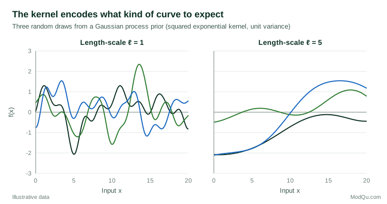
The kernel is where knowledge is represented. The most common choice, the squared exponential kernel, says that the correlation between two function values decays smoothly with the distance between their inputs:
k(x, x′) = σf2 exp(−(x − x′)2 ÷ 2ℓ2)
Here σf sets the typical size of departures from the mean, and the length-scale ℓ sets how far apart two inputs must be before their values become nearly unrelated. A short length-scale allows rapid wiggles; a long one implies slow, gentle change (Figure 1).
Other kernels encode other knowledge. The Matérn family allows rougher functions than the squared exponential, and Stein (1999) argued that it is usually a more realistic default for physical and spatial processes, because the squared exponential assumes an implausible degree of smoothness. Periodic kernels represent repeating seasonal patterns, linear kernels represent trends, and kernels can be added or multiplied to build composite structure, such as a long-term trend plus annual seasonality plus short-term fluctuation (Roberts et al., 2013). In this sense a GP is a flexible way of writing down qualitative knowledge, such as "smooth", "seasonal" or "trending", without committing to a specific equation.
How a Gaussian process learns from data
Suppose we observe noisy values y at inputs x1, …, xn, with independent normal noise of variance σn2. Because everything is jointly normal, Bayes' theorem gives the updated (posterior) distribution of the function at any new input x* in closed form. Writing K for the matrix of kernel values between the observed inputs and k* for the vector of kernel values between x* and the observed inputs, the posterior mean and variance are:
mean(x*) = m(x*) + k*T(K + σn2I)−1(y − m)
var(x*) = k(x*, x*) − k*T(K + σn2I)−1k*
Two features of these formulas matter in practice. First, the posterior mean is a weighted combination of the observations, with nearby, highly correlated observations receiving the most weight. Second, the posterior variance does not depend on the observed values at all, only on where the observations are. It shrinks near data and returns towards the prior variance far from them. This is why a GP's uncertainty bands widen automatically in gaps and beyond the edge of the data.
The kernel's settings, called hyperparameters (σf, ℓ and σn in the example above), are usually estimated by maximising the marginal likelihood, the probability of the observed data averaged over all functions the GP allows. This criterion automatically balances fit against complexity: very wiggly functions can fit the data closely, but they spread their probability over so many possible data sets that they are penalised (Rasmussen & Williams, 2006). A fully Bayesian alternative places priors on the hyperparameters and averages over them, which gives more honest uncertainty when data are limited (Handcock & Stein, 1993; Gelman et al., 2013).
GPs also connect to familiar methods. Kimeldorf and Wahba (1970) showed that smoothing splines arise as posterior means under particular Gaussian process priors, and kriging, the standard interpolation method of geostatistics, is GP prediction under another name (Cressie, 1993). Neal (1996) showed that a neural network with one hidden layer and suitable priors on its weights converges to a Gaussian process as the number of hidden units grows. A GP can therefore be seen as a principled limit of many flexible regression methods.
A worked example: smoothing a brand tracker
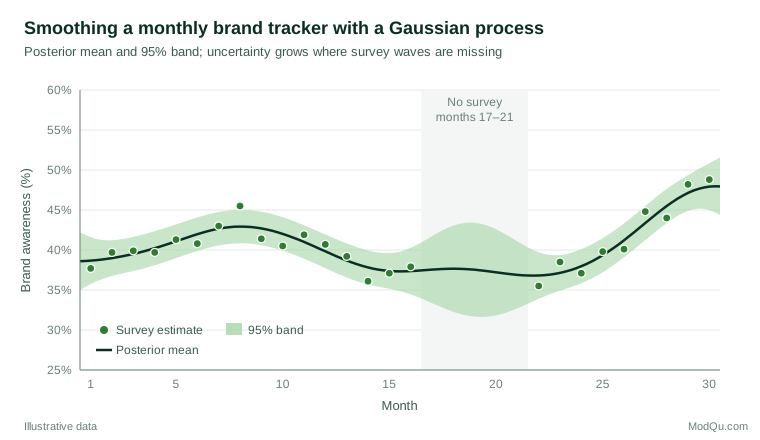
Consider a hypothetical monthly brand-awareness tracker. Each wave interviews 500 people, so a single month's estimate of around 40% has a sampling standard error of about 2.2 percentage points, and a 95% margin of error of roughly ±4.3 points. Over 30 months, 25 waves were fielded; budget cuts meant no fieldwork in months 17 to 21. The raw monthly estimates bounce around, and managers want to know which movements are real.
A GP with a constant mean, a squared exponential kernel with a three-month length-scale, and a noise standard deviation of 2 points (matching the sampling error) gives the result in Figure 2.
Several useful results follow.
- Noise is separated from signal. Where waves are dense, the 95% band for the underlying awareness level is about ±2.1 points, roughly half the ±4.3-point margin of a single wave. The GP borrows strength from neighbouring months, so a one-month jump such as month 8's estimate of 45.5% is treated as partly sampling noise rather than a genuine spike.
- Gaps are filled honestly. In the unfunded months the model interpolates a plausible path, but the band widens to about ±5.9 points in the middle of the gap. The model makes clear that it is guessing more there.
- The ends are less certain. At month 30 the band is about ±2.9 points, wider than in the middle of the series, because there are no later observations to anchor the estimate. This matters, because the most recent point is usually the one managers care about most.
- The trend is readable. The smoothed curve shows a decline from month 8 to month 15 followed by a sustained rise after month 22, a pattern that is hard to see in the raw estimates.
The same approach can be extended. A periodic kernel would capture seasonal patterns, and the noise variance could be set separately for each wave to reflect differing sample sizes or design effects.
Where Gaussian processes are useful
Spatial data and mapping
Geostatistics has used Gaussian processes for decades. Matheron (1963) formalised kriging for estimating ore grades from scattered samples, and Oliver and Webster (1990) describe its use for interpolation in geographical information systems. Diggle et al. (1998) extended GP models to non-normal outcomes such as counts and proportions, under the name model-based geostatistics. In market research, the same tools can map awareness, satisfaction or purchase intention across postal areas, smoothing small local samples while showing where estimates are weak.
Time series and tracking
GPs suit irregularly spaced or gappy time series, where many classical time series methods struggle. Roberts et al. (2013) show how composite kernels capture trends, periodicity and short-term variation, and how the same framework handles missing observations and forecasting with uncertainty.
Computer experiments and simulation models
Many organisations use slow simulation models, for example of supply chains, markets or pricing. Sacks et al. (1989) proposed treating the output of such a model as a Gaussian process, so that a modest number of runs can train a fast "emulator" that predicts the output, with uncertainty, at settings that were never run. Kennedy and O'Hagan (2001) extended this to calibration, combining simulator runs with real observations and including an explicit term for the simulator's own error. Santner et al. (2018) provide a full treatment of design and analysis for such experiments.
Optimisation and experimentation
Because a GP knows where it is uncertain, it can guide where to collect the next observation. Jones et al. (1998) used a GP emulator with an "expected improvement" criterion to find the optimum of expensive functions with few evaluations. This strategy, now known as Bayesian optimisation, is reviewed by Shahriari et al. (2016). In business settings it can help tune prices, promotion levels or campaign settings when each test is costly, by balancing exploration of uncertain options against exploitation of options that already look good.
Classification and other outcomes
GPs are not limited to continuous outcomes. Placing a GP prior on a latent function and passing it through a logistic or probit link gives GP classification, for example of whether a customer will respond. Exact computation is then no longer available, and approximations are needed (Williams & Barber, 1998).
How Gaussian processes compare with other flexible methods
Analysts who need a nonlinear fit have several options: polynomial terms, smoothing splines, generalised additive models, tree ensembles and neural networks. Splines and additive models are fast and familiar and, as noted above, are closely related to GPs (Kimeldorf & Wahba, 1970). Their advantage over a GP is speed and simplicity; their disadvantage is that uncertainty away from the data is usually reported less naturally. Tree ensembles predict well with many inputs but give step-shaped functions and no built-in measure of uncertainty for a single prediction. A GP is most attractive when the data set is small to moderate, when the function is expected to be smooth, and when knowing the uncertainty at each point is part of the question being asked. When there are many thousands of observations and dozens of inputs, other methods are often more practical.
Scaling to large data sets
The main practical drawback of a GP is computation. Fitting requires solving linear systems with an n × n matrix, which takes time proportional to n3 and memory proportional to n2 (Rasmussen & Williams, 2006). A few thousand observations are easy on a laptop; hundreds of thousands are not.
Several families of approximation address this. Low-rank methods summarise the process through a smaller set of representative points or basis functions; examples include the predictive process of Banerjee et al. (2008) and fixed rank kriging (Cressie & Johannesson, 2008). The nearest-neighbour Gaussian process of Datta et al. (2016) conditions each observation only on a small set of nearby neighbours, giving sparse matrices that scale to very large spatial data sets. Lindgren et al. (2011) showed that Gaussian fields with Matérn covariance can be represented as solutions of stochastic partial differential equations, linking them to sparse Gaussian Markov random fields that are fast to compute. Liu et al. (2020) review these and other scalable approaches and the trade-offs between accuracy and speed.
For most survey applications, such as tracking studies with dozens or hundreds of waves, or regional estimates with hundreds of areas, exact GPs are perfectly feasible.
Practical guidance for survey and business data
- Choose the kernel to match what you know. Use smooth kernels for gradually changing quantities, add a periodic component when seasonality is expected, and prefer Matérn kernels when the squared exponential's extreme smoothness is implausible (Stein, 1999).
- Model the noise realistically. For survey estimates, the noise variance can be set from the known sampling variance of each wave or area, including design effects from weighting and clustering. Estimating a single noise term when sample sizes differ greatly can oversmooth large samples and undersmooth small ones.
- Standardise inputs. When several inputs are used, such as price, income and age, rescale them, or use a separate length-scale for each so that the model can learn which inputs matter. A long estimated length-scale suggests that the function changes little along that input.
- Check sensitivity to hyperparameters. With few observations the marginal likelihood can be flat, and different length-scales may fit almost equally well while implying different conclusions. Compare fits, or integrate over hyperparameters in a fully Bayesian analysis (Gelman et al., 2013).
- Evaluate predictive distributions, not just point predictions. Hold out data and score the full predictive distribution with proper scoring rules, which reward both accuracy and well-calibrated uncertainty (Gneiting & Raftery, 2007). A GP that predicts the mean well but gives bands that are too narrow is misleading.
- Respect the outcome's scale. Proportions near 0% or 100% and counts are better modelled on a transformed scale or with a non-normal likelihood (Diggle et al., 1998), so that predictions stay within valid bounds.
Limitations and common mistakes
- Extrapolating far beyond the data. Far from observations, a GP with a constant mean simply reverts to that mean, with wide bands. This is honest, but it is not a forecast of a continuing trend. If a trend is expected to persist, it must be built into the mean function or kernel.
- Treating the bands as the whole story. GP intervals assume the kernel and noise model are right. A poorly chosen kernel can produce bands that are confidently wrong, particularly where the true function changes abruptly. Abrupt changes, such as the effect of a product recall, may need an explicit change-point term.
- Ignoring the cost of size. Naively fitting an exact GP to a very large data set can be slow or impossible; plan for an approximation when n is large.
- Confusing smoothness with causation. A GP can describe how satisfaction varies with price or region in great detail, but like any regression it describes association. Causal claims need a suitable design or additional assumptions.
- Overinterpreting hyperparameters. Length-scales and variances are often only weakly identified, especially together, and should not be read as precise physical quantities (Stein, 1999).
- Over-smoothing real events. A genuine one-month spike caused by a campaign can be smoothed away if the length-scale is long and the noise variance generous. Combine the GP with known event information where it exists.
Gaussian processes as knowledge representation
The appeal of Gaussian processes goes beyond flexible curve fitting. A GP makes three kinds of knowledge explicit. The kernel states prior beliefs about structure: smoothness, periodicity, trend and which inputs matter. The posterior mean states what the data say about the function. The posterior variance states, at every point, how much is still unknown. This makes GPs well suited to tasks in which knowing what is not known matters as much as the best estimate, such as deciding where to collect more survey data, where a regional estimate is too weak to publish, or which pricing scenario deserves a test.
Because GPs are Bayesian, they also combine naturally with other information. Expert beliefs can enter through the mean function or kernel, simulation output can be combined with field data (Kennedy & O'Hagan, 2001), and the predictive distributions can feed directly into decision analysis.
Key takeaways
Gaussian processes let the data determine the shape of a nonlinear relationship, guided by general beliefs encoded in a kernel rather than a fixed formula. They provide smooth estimates with uncertainty that widens honestly in gaps and at the edges of the data, which suits tracking studies, regional mapping, emulation of slow models and the design of costly experiments. Their main costs are computation for large data sets and sensitivity to the choice of kernel and hyperparameters. Used with realistic noise models, sensible kernels and careful checks of predictive performance, they are one of the most useful tools for turning noisy business data into reliable, uncertainty-aware knowledge.
References
Banerjee, S., Gelfand, A. E., Finley, A. O., & Sang, H. (2008). Gaussian predictive process models for large spatial data sets. Journal of the Royal Statistical Society Series B: Statistical Methodology, 70(4), 825–848. https://doi.org/10.1111/j.1467-9868.2008.00663.x
Cressie, N. (1993). Statistics for spatial data (Rev. ed.). Wiley. https://doi.org/10.1002/9781119115151
Cressie, N., & Johannesson, G. (2008). Fixed rank kriging for very large spatial data sets. Journal of the Royal Statistical Society Series B: Statistical Methodology, 70(1), 209–226. https://doi.org/10.1111/j.1467-9868.2007.00633.x
Datta, A., Banerjee, S., Finley, A. O., & Gelfand, A. E. (2016). Hierarchical nearest-neighbor Gaussian process models for large geostatistical datasets. Journal of the American Statistical Association, 111(514), 800–812. https://doi.org/10.1080/01621459.2015.1044091
Diggle, P. J., Tawn, J. A., & Moyeed, R. A. (1998). Model-based geostatistics. Journal of the Royal Statistical Society Series C: Applied Statistics, 47(3), 299–350. https://doi.org/10.1111/1467-9876.00113
Gelman, A., Carlin, J. B., Stern, H. S., Dunson, D. B., Vehtari, A., & Rubin, D. B. (2013). Bayesian data analysis (3rd ed.). Chapman and Hall/CRC. https://doi.org/10.1201/b16018
Gneiting, T., & Raftery, A. E. (2007). Strictly proper scoring rules, prediction, and estimation. Journal of the American Statistical Association, 102(477), 359–378. https://doi.org/10.1198/016214506000001437
Handcock, M. S., & Stein, M. L. (1993). A Bayesian analysis of kriging. Technometrics, 35(4), 403–410. https://doi.org/10.1080/00401706.1993.10485354
Jones, D. R., Schonlau, M., & Welch, W. J. (1998). Efficient global optimization of expensive black-box functions. Journal of Global Optimization, 13(4), 455–492. https://doi.org/10.1023/A:1008306431147
Kennedy, M. C., & O'Hagan, A. (2001). Bayesian calibration of computer models. Journal of the Royal Statistical Society Series B: Statistical Methodology, 63(3), 425–464. https://doi.org/10.1111/1467-9868.00294
Kimeldorf, G. S., & Wahba, G. (1970). A correspondence between Bayesian estimation on stochastic processes and smoothing by splines. The Annals of Mathematical Statistics, 41(2), 495–502. https://doi.org/10.1214/aoms/1177697089
Lindgren, F., Rue, H., & Lindström, J. (2011). An explicit link between Gaussian fields and Gaussian Markov random fields: The stochastic partial differential equation approach. Journal of the Royal Statistical Society Series B: Statistical Methodology, 73(4), 423–498. https://doi.org/10.1111/j.1467-9868.2011.00777.x
Liu, H., Ong, Y.-S., Shen, X., & Cai, J. (2020). When Gaussian process meets big data: A review of scalable GPs. IEEE Transactions on Neural Networks and Learning Systems, 31(11), 4405–4423. https://doi.org/10.1109/TNNLS.2019.2957109
Matheron, G. (1963). Principles of geostatistics. Economic Geology, 58(8), 1246–1266. https://doi.org/10.2113/gsecongeo.58.8.1246
Neal, R. M. (1996). Bayesian learning for neural networks. Springer. https://doi.org/10.1007/978-1-4612-0745-0
O'Hagan, A. (1978). Curve fitting and optimal design for prediction. Journal of the Royal Statistical Society Series B: Statistical Methodology, 40(1), 1–24. https://doi.org/10.1111/j.2517-6161.1978.tb01643.x
Oliver, M. A., & Webster, R. (1990). Kriging: A method of interpolation for geographical information systems. International Journal of Geographical Information Systems, 4(3), 313–332. https://doi.org/10.1080/02693799008941549
Rasmussen, C. E., & Williams, C. K. I. (2006). Gaussian processes for machine learning. MIT Press. https://doi.org/10.7551/mitpress/3206.001.0001
Roberts, S., Osborne, M., Ebden, M., Reece, S., Gibson, N., & Aigrain, S. (2013). Gaussian processes for time-series modelling. Philosophical Transactions of the Royal Society A: Mathematical, Physical and Engineering Sciences, 371(1984), Article 20110550. https://doi.org/10.1098/rsta.2011.0550
Sacks, J., Welch, W. J., Mitchell, T. J., & Wynn, H. P. (1989). Design and analysis of computer experiments. Statistical Science, 4(4), 409–423. https://doi.org/10.1214/ss/1177012413
Santner, T. J., Williams, B. J., & Notz, W. I. (2018). The design and analysis of computer experiments (2nd ed.). Springer. https://doi.org/10.1007/978-1-4939-8847-1
Shahriari, B., Swersky, K., Wang, Z., Adams, R. P., & de Freitas, N. (2016). Taking the human out of the loop: A review of Bayesian optimization. Proceedings of the IEEE, 104(1), 148–175. https://doi.org/10.1109/JPROC.2015.2494218
Stein, M. L. (1999). Interpolation of spatial data: Some theory for kriging. Springer. https://doi.org/10.1007/978-1-4612-1494-6
Williams, C. K. I., & Barber, D. (1998). Bayesian classification with Gaussian processes. IEEE Transactions on Pattern Analysis and Machine Intelligence, 20(12), 1342–1351. https://doi.org/10.1109/34.735807