
Statistics · Bayesian and computational
Dirichlet Process Mixtures for Nonparametric Clustering Knowledge
How Dirichlet process mixture models let the data decide how many clusters there are, how they are fitted, and how to use them responsibly for customer and survey segmentation.
Segmentation is one of the most common tasks in market and survey research. Analysts group customers by needs, respondents by attitudes, or products by usage patterns, and then build strategies around the groups. Almost every clustering method, however, asks an awkward question at the start: how many groups are there? K-means needs K in advance. Finite mixture models need the number of components, usually chosen by refitting the model many times and comparing information criteria. Whatever number is chosen is then treated as if it were known, and the uncertainty about it disappears from the final report.
Dirichlet process mixture (DPM) models take a different approach. They come from Bayesian nonparametric statistics, in which the number of parameters is allowed to grow with the data. A DPM assumes, in principle, an unlimited number of possible clusters, of which only a finite number will be occupied by any data set. The model then infers how many clusters the data support, which observations belong together, and how uncertain both conclusions are. This article explains the idea, the main computational methods, and the practical value and limits of DPMs for building knowledge about segments.
From finite mixtures to infinite ones
A finite mixture model assumes that each observation comes from one of K subpopulations, each with its own distribution, for example a multivariate normal with its own mean and covariance. The mixture density is
p(x) = π1f(x | θ1) + π2f(x | θ2) + … + πKf(x | θK)
where the weights πk sum to one and θk are the parameters of each component. Finite mixtures are well established for clustering, density estimation and market segmentation (McLachlan & Peel, 2000; Wedel & Kamakura, 2000), and model-based clustering with a criterion such as the Bayesian information criterion is a standard way to choose K (Fraley & Raftery, 2002).
A Dirichlet process mixture lets K go to infinity, but in a controlled way. Instead of a fixed set of weights, it places a prior on an infinite sequence of weights that decline quickly, so that a few components carry most of the probability. The prior is the Dirichlet process, introduced by Ferguson (1973) as a probability distribution over probability distributions. Antoniak (1974) extended it to mixtures of distributions, but the approach became practical only with the Markov chain Monte Carlo methods of the 1990s (Escobar & West, 1995).
Three ways to picture the Dirichlet process
The Dirichlet process has two ingredients: a base distribution G0, which describes typical cluster parameters, and a concentration parameter α, which controls how many clusters tend to appear. Three equivalent constructions explain how it behaves.
The stick-breaking construction
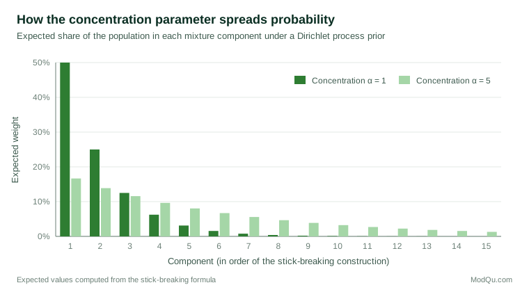
Imagine a stick of length one. Break off a random fraction V1 drawn from a Beta(1, α) distribution; that piece is the weight of the first component. Break the same fraction type from what remains to get the second weight, and so on for ever. Each component receives parameters drawn from G0. The expected weights decline geometrically: with α = 1, the first component expects half the stick, the second a quarter, the third an eighth. With larger α, each break takes a smaller piece and the mass spreads over many more components (Figure 1). Ishwaran and James (2001) built an efficient sampling method directly on this construction.
The Pólya urn and the Chinese restaurant
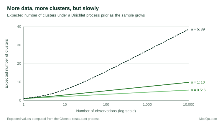
Blackwell and MacQueen (1973) showed that the Dirichlet process can also be described by an urn scheme, often retold as the "Chinese restaurant process". Customers enter one at a time. Each new customer sits at an occupied table with probability proportional to the number of people already there, or starts a new table with probability proportional to α. Tables are clusters. The scheme makes two properties visible. First, it is "rich get richer": large clusters attract more members. Second, new clusters keep appearing, but more and more slowly. The expected number of clusters grows roughly as α times the logarithm of the sample size (Figure 2). With α = 1, a sample of 10,000 is expected to occupy about 10 clusters under the prior.
The limit of finite mixtures
A third view treats the DPM as the limit of a finite mixture with K components and symmetric Dirichlet weights as K becomes very large. This view connects DPMs to familiar finite mixtures and explains why they behave similarly when the data contain a few well-separated groups.
Fitting a Dirichlet process mixture
The posterior distribution of a DPM cannot be written in closed form, so it is approximated by simulation or optimisation.
Gibbs sampling over cluster assignments. Escobar and West (1995) and MacEachern and Müller (1998) developed samplers that repeatedly reassign each observation to an existing cluster or to a new one, using the Chinese restaurant probabilities weighted by how well the observation fits each cluster. Neal (2000) reviewed and extended these algorithms, including versions for base distributions that are not conjugate to the data model. These samplers are the standard tools in statistical software.
Truncated stick-breaking. Ishwaran and James (2001) showed that truncating the stick-breaking construction at a generous number of components, say 30 or 50, gives an excellent approximation that can be fitted with ordinary blocked Gibbs sampling. Components that the data do not need receive negligible weight.
Variational inference. For large data sets, Blei and Jordan (2006) developed a variational algorithm that replaces sampling with optimisation of an approximating distribution. It is much faster but tends to understate uncertainty, a general property of variational methods.
Whatever the algorithm, the output is not a single clustering but a posterior distribution over clusterings. Each draw assigns observations to clusters, and the number of occupied clusters varies from draw to draw. Two summaries are especially useful. The posterior distribution of the number of clusters shows how strongly the data support, say, four segments rather than five. The posterior similarity matrix records, for each pair of observations, the proportion of draws in which they share a cluster; it shows which segment memberships are firm and which are ambiguous. Wade and Ghahramani (2018) proposed principled ways to choose a single representative clustering from this distribution and to express the uncertainty around it.
A worked example: attitudinal segments
Consider a hypothetical survey of 1,200 customers who rate the importance of 12 product attributes. After reducing the ratings to a few attitude scores, an analyst fits a DPM of multivariate normal distributions with a concentration parameter that is itself given a prior, as recommended by Escobar and West (1995), so that the data can inform how many clusters are likely.
The posterior might put 55% probability on five occupied clusters, 30% on six and 15% on seven or more. Inspection shows four large segments, labelled price-focused, quality-focused, convenience-focused and brand-loyal, each containing between 180 and 400 customers, and a fifth segment of about 70 customers who care strongly about sustainability. The sixth cluster, when it appears, splits the quality-focused group into two similar halves. The posterior similarity matrix shows that 85% of customers are allocated to the same segment in more than 90% of draws, while about 15%, mostly between the quality-focused and brand-loyal groups, move back and forth.
This is richer knowledge than a single k-means solution. The analyst can report that five segments are well supported, that a further split is possible but uncertain, that a small sustainability segment exists, and which customers sit on boundaries. Targeting decisions for boundary customers can take that uncertainty into account.
How DPMs compare with other clustering methods
| Method | Number of clusters | Uncertainty about membership | Main weakness |
|---|---|---|---|
| K-means | Fixed in advance | None; each case gets one cluster | Assumes round clusters of similar size |
| Finite mixture with an information criterion | Chosen by refitting for several K | Membership probabilities given the chosen K | Ignores uncertainty about K |
| Hierarchical clustering | Chosen by cutting a tree | None | Results depend on linkage and distance choices |
| Dirichlet process mixture | Inferred, with a posterior distribution | Full posterior, including co-clustering probabilities | Sensitive to priors; computationally heavier |
K-means remains useful for quick exploration and very large data sets, and its centroids are easy to explain to managers who need a simple description of each group (Wedel & Kamakura, 2000). Finite mixtures with the Bayesian information criterion are a sound default when the data contain a few clear groups. The extra value of a DPM lies in situations where the number of segments is genuinely uncertain, where small but distinct groups may exist, or where the analyst needs to show decision-makers how firm each segment is. In those situations, presenting a single partition as if it were certain overstates what the data can support.
A further practical advantage is that a DPM produces a full predictive density for new observations. That makes it useful beyond segmentation: for example, to flag a new customer whose profile fits poorly with every existing segment, or to estimate how many customers in a population are likely to fall into a rare group. The same density can also be used to simulate realistic synthetic customers for testing targeting rules before they are applied to real people.
Extensions
The basic DPM has been extended in many directions useful for business and survey data.
- Hierarchical Dirichlet processes share clusters across groups, such as countries, stores or survey waves, while letting each group weight them differently (Teh et al., 2006). A segment can then be recognised in every market even if its size varies.
- Pitman-Yor processes add a second parameter that produces more small clusters and heavier-tailed cluster sizes, often a better fit for data such as product categories or words in open-ended answers (Pitman & Yor, 1997).
- Variable selection within DPMs identifies which variables actually distinguish clusters, avoiding segments driven by noise variables (Kim et al., 2006).
- Mixtures of finite mixtures place a prior directly on the number of components and can be fitted with similar algorithms (Miller & Harrison, 2018).
- Bayesian marketing models use DPMs to describe heterogeneity in consumer preferences, for example in choice models, without forcing preferences into a normal distribution (Rossi & Allenby, 2003).
Broader introductions to these models are given by Gershman and Blei (2012) and, at a more technical level, Ghosal and van der Vaart (2017).
Limitations and common mistakes
DPMs are attractive, but they are not a way of discovering the "true" number of segments automatically.
- The prior matters. The concentration parameter and the base distribution strongly influence how many clusters appear. A base distribution that allows very tight clusters will produce many small ones. Sensitivity analysis over reasonable priors is essential (Gelman et al., 2013).
- The number of clusters is not consistently estimated. Miller and Harrison (2018) showed that, when data truly come from a finite mixture, the DPM posterior on the number of clusters does not settle on the correct value as the sample grows; it tends to add small extra clusters. DPMs are excellent for density estimation and for finding the main groups, but small clusters should be interpreted with caution.
- Model misspecification creates clusters. If the real groups are skewed or heavy-tailed but each component is normal, the model will use several components to describe one real group. Using flexible component distributions or merging similar components helps.
- Label switching. Cluster labels have no fixed meaning across posterior draws, so averaging "cluster 3" over draws is meaningless. Summaries should use label-invariant quantities such as the similarity matrix.
- Computation and convergence. Samplers can get stuck in poor configurations. Running several chains from different starting points and checking that they agree is basic good practice.
- Statistical clusters are not market segments. A segment must also be substantial, reachable and actionable. Cluster stability checks, such as resampling (Hennig, 2007), and business review remain necessary.
Practical guidance
- Prepare the variables. Standardise inputs and reduce many correlated ratings to a smaller set of scores, so that clusters reflect meaningful differences.
- Put a prior on α. A Gamma prior on the concentration parameter lets the data inform the expected number of clusters instead of fixing it.
- Check sensitivity. Refit with different priors and base distributions and report how the main segments change.
- Report uncertainty. Present the posterior distribution of the number of clusters, segment sizes with intervals, and the share of observations with uncertain membership.
- Validate externally. Check that segments differ on variables not used in the clustering, such as spending or retention, and that they reappear in a new sample.
- Compare with simpler methods. If a finite mixture chosen by an information criterion gives the same main segments, that agreement strengthens the conclusion (Frühwirth-Schnatter, 2006).
Key takeaways
Dirichlet process mixtures remove the need to fix the number of clusters in advance by placing a prior on an unlimited number of components and letting the data decide how many are used. Through the stick-breaking and Chinese restaurant constructions, the concentration parameter controls how readily new clusters form. Fitted by Gibbs sampling or variational methods, a DPM produces a distribution over clusterings that shows both the main segments and the uncertainty around them. Used with sensible priors, careful checks and business judgement, it turns segmentation from a single guessed partition into a reasoned statement about what groups the data support.
References
Antoniak, C. E. (1974). Mixtures of Dirichlet processes with applications to Bayesian nonparametric problems. The Annals of Statistics, 2(6), 1152–1174. https://doi.org/10.1214/aos/1176342871
Blackwell, D., & MacQueen, J. B. (1973). Ferguson distributions via Pólya urn schemes. The Annals of Statistics, 1(2), 353–355. https://doi.org/10.1214/aos/1176342372
Blei, D. M., & Jordan, M. I. (2006). Variational inference for Dirichlet process mixtures. Bayesian Analysis, 1(1), 121–143. https://doi.org/10.1214/06-BA104
Escobar, M. D., & West, M. (1995). Bayesian density estimation and inference using mixtures. Journal of the American Statistical Association, 90(430), 577–588. https://doi.org/10.1080/01621459.1995.10476550
Ferguson, T. S. (1973). A Bayesian analysis of some nonparametric problems. The Annals of Statistics, 1(2), 209–230. https://doi.org/10.1214/aos/1176342360
Fraley, C., & Raftery, A. E. (2002). Model-based clustering, discriminant analysis, and density estimation. Journal of the American Statistical Association, 97(458), 611–631. https://doi.org/10.1198/016214502760047131
Frühwirth-Schnatter, S. (2006). Finite mixture and Markov switching models. Springer. https://doi.org/10.1007/978-0-387-35768-3
Gelman, A., Carlin, J. B., Stern, H. S., Dunson, D. B., Vehtari, A., & Rubin, D. B. (2013). Bayesian data analysis (3rd ed.). Chapman and Hall/CRC. https://doi.org/10.1201/b16018
Gershman, S. J., & Blei, D. M. (2012). A tutorial on Bayesian nonparametric models. Journal of Mathematical Psychology, 56(1), 1–12. https://doi.org/10.1016/j.jmp.2011.08.004
Ghosal, S., & van der Vaart, A. (2017). Fundamentals of nonparametric Bayesian inference. Cambridge University Press. https://doi.org/10.1017/9781139029834
Hennig, C. (2007). Cluster-wise assessment of cluster stability. Computational Statistics & Data Analysis, 52(1), 258–271. https://doi.org/10.1016/j.csda.2006.11.025
Ishwaran, H., & James, L. F. (2001). Gibbs sampling methods for stick-breaking priors. Journal of the American Statistical Association, 96(453), 161–173. https://doi.org/10.1198/016214501750332758
Kim, S., Tadesse, M. G., & Vannucci, M. (2006). Variable selection in clustering via Dirichlet process mixture models. Biometrika, 93(4), 877–893. https://doi.org/10.1093/biomet/93.4.877
MacEachern, S. N., & Müller, P. (1998). Estimating mixture of Dirichlet process models. Journal of Computational and Graphical Statistics, 7(2), 223–238. https://doi.org/10.1080/10618600.1998.10474772
McLachlan, G., & Peel, D. (2000). Finite mixture models. Wiley. https://doi.org/10.1002/0471721182
Miller, J. W., & Harrison, M. T. (2018). Mixture models with a prior on the number of components. Journal of the American Statistical Association, 113(521), 340–356. https://doi.org/10.1080/01621459.2016.1255636
Neal, R. M. (2000). Markov chain sampling methods for Dirichlet process mixture models. Journal of Computational and Graphical Statistics, 9(2), 249–265. https://doi.org/10.1080/10618600.2000.10474879
Pitman, J., & Yor, M. (1997). The two-parameter Poisson-Dirichlet distribution derived from a stable subordinator. The Annals of Probability, 25(2), 855–900. https://doi.org/10.1214/aop/1024404422
Rossi, P. E., & Allenby, G. M. (2003). Bayesian statistics and marketing. Marketing Science, 22(3), 304–328. https://doi.org/10.1287/mksc.22.3.304.17739
Teh, Y. W., Jordan, M. I., Beal, M. J., & Blei, D. M. (2006). Hierarchical Dirichlet processes. Journal of the American Statistical Association, 101(476), 1566–1581. https://doi.org/10.1198/016214506000000302
Wade, S., & Ghahramani, Z. (2018). Bayesian cluster analysis: Point estimation and credible balls (with discussion). Bayesian Analysis, 13(2), 559–626. https://doi.org/10.1214/17-BA1073
Wedel, M., & Kamakura, W. A. (2000). Market segmentation: Conceptual and methodological foundations (2nd ed.). Springer. https://doi.org/10.1007/978-1-4615-4651-1