
Statistics · Bayesian and computational
Variational Inference Methods for Scalable Bayesian Knowledge
How variational inference turns Bayesian computation into optimisation so that models can be fitted to very large data sets, and what is lost in the approximation.
Bayesian statistics offers a coherent way to learn from data: start with prior beliefs about unknown quantities, combine them with the likelihood of the observed data, and obtain a posterior distribution that expresses what is known and how uncertain it is. The difficulty has always been computation. For all but the simplest models, the posterior cannot be calculated exactly. Markov chain Monte Carlo (MCMC) solved that problem for a generation of statisticians by drawing samples from the posterior, but MCMC can be slow when data sets have millions of records or models have millions of parameters.
Variational inference (VI) takes a different route. Instead of sampling from the posterior, it picks the closest member of a simpler family of distributions and uses that as an approximation. Finding the closest member is an optimisation problem, and optimisation scales to very large problems. VI is now at the heart of topic models for text, large hierarchical models in marketing, and the probabilistic parts of modern machine learning. This article explains how VI works, where it is reliable, and where its speed comes at the cost of misleading answers.
The computational problem
For parameters θ and data y, Bayes' theorem gives the posterior
p(θ | y) = p(y | θ) p(θ) ÷ p(y)
The denominator p(y), the marginal likelihood, is an integral over all parameter values. In high dimensions it is usually impossible to compute, and without it the posterior is known only up to a constant. Analytic approximations, such as the Laplace approximation around the posterior mode (Tierney & Kadane, 1986), work when the posterior is close to normal. Simulation methods avoid the integral altogether: the Metropolis algorithm (Metropolis et al., 1953), Gibbs sampling (Geman & Geman, 1984) and their application to Bayesian statistics (Gelfand & Smith, 1990) made it possible to fit complex models by drawing dependent samples whose distribution converges to the posterior (Robert & Casella, 2004). Modern samplers in software such as Stan (Carpenter et al., 2017) are efficient and come with good diagnostics (Vehtari et al., 2021), but each iteration requires a pass through the data, and thousands of iterations may be needed.
Inference as optimisation
Variational inference, which grew out of statistical physics and was developed for graphical models in machine learning (Jordan et al., 1999), reframes the problem. Choose a family Q of tractable distributions, for example independent normal distributions for each parameter. Then find the member q(θ) of that family that is closest to the posterior, measuring closeness by the Kullback-Leibler divergence (Kullback & Leibler, 1951):
KL(q ‖ p) = Eq[ log q(θ) − log p(θ | y) ]
This divergence still involves the unknown posterior, but a rearrangement removes the problem. Minimising KL(q ‖ p) is equivalent to maximising the evidence lower bound (ELBO):
ELBO(q) = Eq[ log p(y, θ) ] − Eq[ log q(θ) ]
The ELBO uses only the joint density of data and parameters, which is easy to evaluate. Its name comes from the fact that it is always less than or equal to log p(y), the log evidence. Maximising it therefore both improves the approximation and gives a lower bound on the evidence that can be used, with care, to compare models (Blei et al., 2017).
An intuition for the ELBO
The two terms of the ELBO pull in opposite directions, which helps explain how the method behaves. The first term, the expected log joint density, rewards approximations that put their probability where the data and prior together are most plausible; on its own it would shrink q to a single point at the posterior mode. The second term, the entropy of q, rewards spreading probability out. The optimum balances fit against spread. Because the expectation is taken under q, regions where q puts no probability cost nothing, even if the posterior has substantial mass there. That asymmetry is the source of the characteristic behaviour of VI: it tends to find a compact region of high posterior density and stay there.
The ELBO also connects VI to the expectation-maximisation algorithm. EM can be seen as maximising the same bound when the approximating distribution for the latent variables is allowed to equal their exact conditional posterior; variational EM simply restricts that distribution to a tractable family when the exact one is unavailable (Jordan et al., 1999). For analysts familiar with mixture models fitted by EM, this is a helpful bridge.
Mean-field variational inference
The most common choice of family is the mean-field family, in which the parameters are treated as independent in the approximation:
q(θ) = q1(θ1) × q2(θ2) × … × qm(θm)
For many models built from conjugate exponential-family components, the optimal form of each factor can be derived exactly, and the ELBO can be maximised by updating each factor in turn while holding the others fixed, a procedure called coordinate ascent variational inference. Each update resembles a step of Gibbs sampling, but it replaces random draws with expectations. Ormerod and Wand (2010) give an accessible statistical introduction, and Wand et al. (2011) extend the approach to more elaborate distributions. Wainwright and Jordan (2008) provide the deeper theory linking VI to exponential families and convex optimisation.
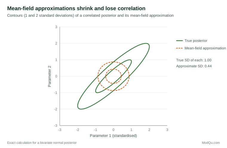
The independence assumption has a cost, illustrated in Figure 1. When two parameters are strongly correlated in the posterior, as regression coefficients on related predictors often are, the mean-field approximation cannot represent the correlation. Because it minimises KL(q ‖ p), which heavily penalises putting probability where the posterior has little, it chooses a narrow distribution that sits inside the posterior. In the bivariate normal case with correlation 0.9, the approximation gets the posterior means exactly right, but each marginal standard deviation is only about 0.44 of the true value.
The direction of the divergence matters
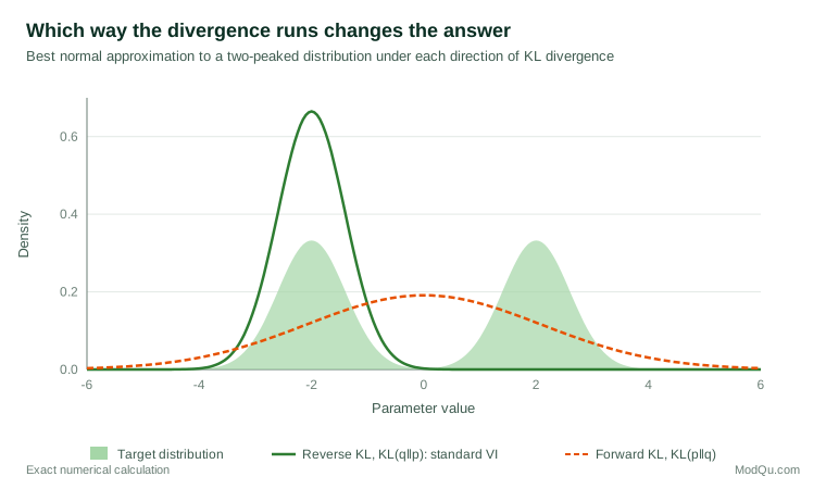
KL divergence is not symmetric. Standard VI minimises the "reverse" divergence KL(q ‖ p). Its alternative, KL(p ‖ q), the "forward" divergence, penalises missing any region where the posterior has probability, and leads to approximations that spread out to cover everything. The difference is stark when the posterior has more than one peak (Figure 2). The reverse divergence locks on to one mode and ignores the other; the forward divergence places a broad distribution over both, with much of its probability in the empty valley between them. Neither is a good summary of a two-peaked posterior, but the reverse divergence is the more dangerous for decision-making because it reports false confidence. Methods such as expectation propagation minimise local versions of the forward divergence and tend to give wider, more cautious answers (Zhang et al., 2019).
Making variational inference scale
Two developments turned VI into a tool for very large data sets.
Stochastic optimisation. Instead of computing the ELBO's gradient from all the data at every step, stochastic variational inference estimates it from small random subsets of the data and takes many cheap, noisy steps. Convergence follows from the classical theory of stochastic approximation (Robbins & Monro, 1951). This allows a model to be fitted to millions of documents or customers with each step touching only a few hundred of them (Hoffman et al., 2013), an approach that made topic models such as latent Dirichlet allocation (Blei et al., 2003) practical on whole archives of text.
Black-box and automatic methods. Early VI required model-specific mathematical derivations. Newer methods estimate gradients by Monte Carlo sampling from q and use automatic differentiation, so that one algorithm works for a wide range of models. The reparameterisation approach, popularised in variational autoencoders, writes a draw from q as a smooth transformation of fixed random noise, which gives low-variance gradient estimates (Kingma & Welling, 2019). Probabilistic programming systems now offer automatic VI alongside MCMC, letting analysts try both on the same model.
Richer families also reduce the cost of the mean-field assumption. Full-rank normal approximations capture correlations among parameters; mixtures and normalising flows, which transform a simple distribution through a series of invertible functions, can represent skewed and multimodal shapes (Zhang et al., 2019).
How variational inference compares with other methods
| Feature | MCMC | Variational inference | Laplace and INLA |
|---|---|---|---|
| Basic idea | Draw dependent samples from the posterior | Optimise the closest tractable distribution | Normal or nested normal approximations around the mode |
| Accuracy | Exact in the limit of long runs | Approximate; error usually unknown | Very accurate for latent Gaussian models; poor for multimodal posteriors |
| Typical speed | Slow for large data | Fast; scales to millions of observations | Very fast for suitable models |
| Uncertainty | Reliable if chains converge | Often too narrow | Good within its model class |
| Diagnostics | Well developed | Developing | Model-specific |
Integrated nested Laplace approximations (INLA) deserve special mention for survey and spatial work. For the large class of latent Gaussian models, which includes many hierarchical, small area, spatial and time-series models, INLA computes accurate approximations to posterior marginals in seconds rather than hours, using nested Laplace approximations rather than a variational family (Rue et al., 2009). When a model fits that class, INLA is often preferable to both MCMC and VI. When it does not, VI is the more general fast option.
The choice between methods is therefore practical rather than ideological. MCMC remains the gold standard for moderate problems where accurate uncertainty is essential. VI is the tool for very large data, very large models or rapid iteration. INLA is the tool for latent Gaussian models of any size. Many analysts use more than one, letting a fast method guide model building and a slower method confirm the final results.
Variational inference in business and survey applications
VI is attractive wherever the data are large, the model is hierarchical and results are needed quickly.
- Choice and preference models. Braun and McAuliffe (2010) developed variational methods for hierarchical discrete choice models of the kind used in conjoint analysis and marketing, and showed that they give estimates close to MCMC in a fraction of the time. Bayesian hierarchical models have long been central to marketing research (Rossi & Allenby, 2003), and VI makes them feasible at the scale of loyalty card and online data.
- Text from open-ended questions. Topic models fitted by VI summarise thousands of verbatim survey responses or reviews into themes.
- Large-scale personalisation. Recommendation and targeting systems use VI to estimate customer-level parameters for millions of customers.
- Rapid iteration. Even when MCMC will be used for the final analysis, VI provides fast approximate fits for exploring model specifications.
A worked example: a hierarchical satisfaction model
Consider a hypothetical retailer with satisfaction ratings from 2 million customers across 3,000 stores. The analyst fits a hierarchical model in which each store has its own mean satisfaction and its own effect of waiting time, with store effects drawn from a common distribution. MCMC on the full data would take many hours; mean-field VI with stochastic optimisation converges in minutes.
The analyst then fits the model by MCMC to a random 5% of stores to check the approximation. In this illustration, the two methods agree closely on the average effect of waiting time and on the ranking of stores. However, the VI intervals for individual store means are about 30% narrower than the MCMC intervals, and the between-store standard deviation is slightly underestimated. The analyst therefore uses VI estimates to rank stores and screen for problems, but reports uncertainty for individual stores using the MCMC results, or uses a full-rank approximation that captures the correlation between store means and the hyperparameters.
The comparison also reveals where the approximation matters for decisions. Ranking stores from best to worst depends mainly on the estimated means, which VI gets right. Deciding whether a particular store is significantly below the chain average depends on its interval, which VI makes too narrow: in this illustration, 140 stores appear clearly below average under VI but only 95 under MCMC. A manager acting on the VI intervals alone would send improvement teams to 45 stores whose apparent problems are within the range of normal variation. The lesson is not that VI is unusable, but that its outputs should be matched to the decisions they support.
Is the approximation good enough?
Because VI is an approximation of unknown quality, checking it is part of the job.
- Compare with MCMC on a subset or a smaller model. If both give similar means and intervals, VI can be trusted for the full analysis.
- Use diagnostics. Importance-sampling diagnostics can show when the approximation is far from the posterior, and simulation-based calibration can test whether intervals have the right coverage.
- Examine the ELBO trace. It should rise and stabilise; erratic behaviour suggests a learning rate that is too high or a poorly specified model.
- Check predictions. Posterior predictive checks reveal whether the approximate posterior produces data that look like the real data (Gelman et al., 2013).
On the theoretical side, Wang and Blei (2019) showed that variational Bayes posteriors concentrate around the true parameter values as data grow, under regularity conditions, which supports the use of VI for point estimates in large samples. The theory says less about whether the spread of the approximation is right, and that is where most practical problems lie.
Limitations and common mistakes
- Understated uncertainty. Mean-field VI typically produces intervals that are too narrow, especially for correlated parameters and variance components. Using VI intervals as if they were exact posterior intervals is the most common error.
- Local optima. The ELBO can have many local maxima. Different starting points can give different answers, particularly in mixture and clustering models. Multiple runs are advisable.
- Model comparison by ELBO. The ELBO is a lower bound with an unknown gap that differs between models, so comparing models by ELBO alone can mislead.
- Hidden defaults. Automatic VI in software makes choices about families, learning rates and convergence tolerances that affect results; these should be reported.
Practical guidance
- Start with the model, not the algorithm. Write down the model and priors as for any Bayesian analysis.
- Use MCMC when it is feasible. For moderate data and models, modern MCMC gives more reliable uncertainty. Use VI when speed or scale makes MCMC impractical.
- Validate VI against MCMC on a subset, a simplified model or simulated data, and report the comparison.
- Prefer richer families (full-rank or flows) when correlations or uncertainty matter.
- Interpret intervals cautiously and say in reports that they come from an approximation.
Key takeaways
Variational inference makes Bayesian modelling feasible at large scale by replacing sampling with optimisation: it finds the member of a tractable family that is closest to the posterior by maximising the evidence lower bound. Stochastic and automatic methods let it handle millions of observations and very general models. The price is approximation error, most often in the form of overconfident intervals and missed correlations or modes. Used for speed and exploration, checked against MCMC where possible and reported honestly, VI extends the reach of Bayesian knowledge to data sets that would otherwise be out of range.
References
Blei, D. M., Kucukelbir, A., & McAuliffe, J. D. (2017). Variational inference: A review for statisticians. Journal of the American Statistical Association, 112(518), 859–877. https://doi.org/10.1080/01621459.2017.1285773
Blei, D. M., Ng, A. Y., & Jordan, M. I. (2003). Latent Dirichlet allocation. Journal of Machine Learning Research, 3, 993–1022.
Braun, M., & McAuliffe, J. (2010). Variational inference for large-scale models of discrete choice. Journal of the American Statistical Association, 105(489), 324–335. https://doi.org/10.1198/jasa.2009.tm08030
Carpenter, B., Gelman, A., Hoffman, M. D., Lee, D., Goodrich, B., Betancourt, M., Brubaker, M., Guo, J., Li, P., & Riddell, A. (2017). Stan: A probabilistic programming language. Journal of Statistical Software, 76(1), 1–32. https://doi.org/10.18637/jss.v076.i01
Gelfand, A. E., & Smith, A. F. M. (1990). Sampling-based approaches to calculating marginal densities. Journal of the American Statistical Association, 85(410), 398–409. https://doi.org/10.1080/01621459.1990.10476213
Gelman, A., Carlin, J. B., Stern, H. S., Dunson, D. B., Vehtari, A., & Rubin, D. B. (2013). Bayesian data analysis (3rd ed.). Chapman and Hall/CRC. https://doi.org/10.1201/b16018
Geman, S., & Geman, D. (1984). Stochastic relaxation, Gibbs distributions, and the Bayesian restoration of images. IEEE Transactions on Pattern Analysis and Machine Intelligence, PAMI-6(6), 721–741. https://doi.org/10.1109/TPAMI.1984.4767596
Hoffman, M. D., Blei, D. M., Wang, C., & Paisley, J. (2013). Stochastic variational inference. Journal of Machine Learning Research, 14, 1303–1347.
Jordan, M. I., Ghahramani, Z., Jaakkola, T. S., & Saul, L. K. (1999). An introduction to variational methods for graphical models. Machine Learning, 37(2), 183–233. https://doi.org/10.1023/A:1007665907178
Kingma, D. P., & Welling, M. (2019). An introduction to variational autoencoders. Foundations and Trends in Machine Learning, 12(4), 307–392. https://doi.org/10.1561/2200000056
Kullback, S., & Leibler, R. A. (1951). On information and sufficiency. The Annals of Mathematical Statistics, 22(1), 79–86. https://doi.org/10.1214/aoms/1177729694
Metropolis, N., Rosenbluth, A. W., Rosenbluth, M. N., Teller, A. H., & Teller, E. (1953). Equation of state calculations by fast computing machines. The Journal of Chemical Physics, 21(6), 1087–1092. https://doi.org/10.1063/1.1699114
Ormerod, J. T., & Wand, M. P. (2010). Explaining variational approximations. The American Statistician, 64(2), 140–153. https://doi.org/10.1198/tast.2010.09058
Robbins, H., & Monro, S. (1951). A stochastic approximation method. The Annals of Mathematical Statistics, 22(3), 400–407. https://doi.org/10.1214/aoms/1177729586
Robert, C. P., & Casella, G. (2004). Monte Carlo statistical methods (2nd ed.). Springer. https://doi.org/10.1007/978-1-4757-4145-2
Rossi, P. E., & Allenby, G. M. (2003). Bayesian statistics and marketing. Marketing Science, 22(3), 304–328. https://doi.org/10.1287/mksc.22.3.304.17739
Rue, H., Martino, S., & Chopin, N. (2009). Approximate Bayesian inference for latent Gaussian models by using integrated nested Laplace approximations. Journal of the Royal Statistical Society Series B: Statistical Methodology, 71(2), 319–392. https://doi.org/10.1111/j.1467-9868.2008.00700.x
Tierney, L., & Kadane, J. B. (1986). Accurate approximations for posterior moments and marginal densities. Journal of the American Statistical Association, 81(393), 82–86. https://doi.org/10.1080/01621459.1986.10478240
Vehtari, A., Gelman, A., Simpson, D., Carpenter, B., & Bürkner, P.-C. (2021). Rank-normalization, folding, and localization: An improved R̂ for assessing convergence of MCMC (with discussion). Bayesian Analysis, 16(2), 667–718. https://doi.org/10.1214/20-BA1221
Wainwright, M. J., & Jordan, M. I. (2008). Graphical models, exponential families, and variational inference. Foundations and Trends in Machine Learning, 1(1–2), 1–305. https://doi.org/10.1561/2200000001
Wand, M. P., Ormerod, J. T., Padoan, S. A., & Frühwirth, R. (2011). Mean field variational Bayes for elaborate distributions. Bayesian Analysis, 6(4), 847–900. https://doi.org/10.1214/11-BA631
Wang, Y., & Blei, D. M. (2019). Frequentist consistency of variational Bayes. Journal of the American Statistical Association, 114(527), 1147–1161. https://doi.org/10.1080/01621459.2018.1473776
Zhang, C., Bütepage, J., Kjellström, H., & Mandt, S. (2019). Advances in variational inference. IEEE Transactions on Pattern Analysis and Machine Intelligence, 41(8), 2008–2026. https://doi.org/10.1109/TPAMI.2018.2889774