
Surveys · Nonresponse, weighting and data quality
Survey Weighting Methods: Post-Stratification, Raking and Calibration
Survey weights make a sample represent the population it was drawn from. This article explains how weights are built, from design weights through nonresponse adjustment to post-stratification, raking and calibration, and discusses the choices and trade-offs involved.
Almost every survey sample differs from its population in some way. Some groups were deliberately sampled at higher rates; some responded more readily than others; some were missed by the sampling frame. If results are calculated as though every respondent counted equally, these differences pass straight into the estimates. Survey weights correct for them by giving each respondent a value that indicates how many members of the population they represent (Kalton & Flores-Cervantes, 2003; Valliant et al., 2018).
Weighting is usually done in stages. A design weight reflects each respondent's chance of selection. A nonresponse adjustment compensates for differences in response between groups. A final adjustment aligns the weighted sample with known population totals, using post-stratification, raking or, more generally, calibration (Haziza & Beaumont, 2017). This article explains each stage, with most attention on the final adjustment methods, and discusses the trade-offs they involve.
Stage one: design weights
In a probability sample, each member of the population has a known chance of selection. The design weight is the inverse of that probability. If one in every 500 households is selected, each selected household has a design weight of 500: it represents itself and 499 others. When some groups are sampled at higher rates, for example to ensure enough cases in small regions, their design weights are smaller, so that they do not count for more than their share of the population (Kish, 1992; Lohr, 2021).
Design weights also handle selection within households. If one adult is selected at random from each sampled household, an adult in a household with three adults had a one-in-three chance of selection once the household was chosen, so their weight is three times that of an adult living alone.
Stage two: nonresponse adjustment
Not all selected people respond. If response differs between groups, respondents will not represent the population even with correct design weights. A common approach divides the sample into weighting classes using variables known for both respondents and nonrespondents, such as region or type of area, and increases the weights of respondents in each class so that they represent the nonrespondents in that class (Kalton & Flores-Cervantes, 2003).
An alternative is to model each sampled person's probability of responding using available information, and to divide the design weight by the estimated response propensity. Classes are often formed by grouping people with similar propensities. Little (1986) showed that nonresponse adjustments reduce bias when the variables used are related to both response and the survey outcomes, and Little and Vartivarian (2005) showed that such adjustments need not increase variance when the variables are strongly related to the outcomes. Brick (2013) reviewed the evidence and concluded that the choice of variables matters far more than the choice of method.
Stage three: adjusting to population totals
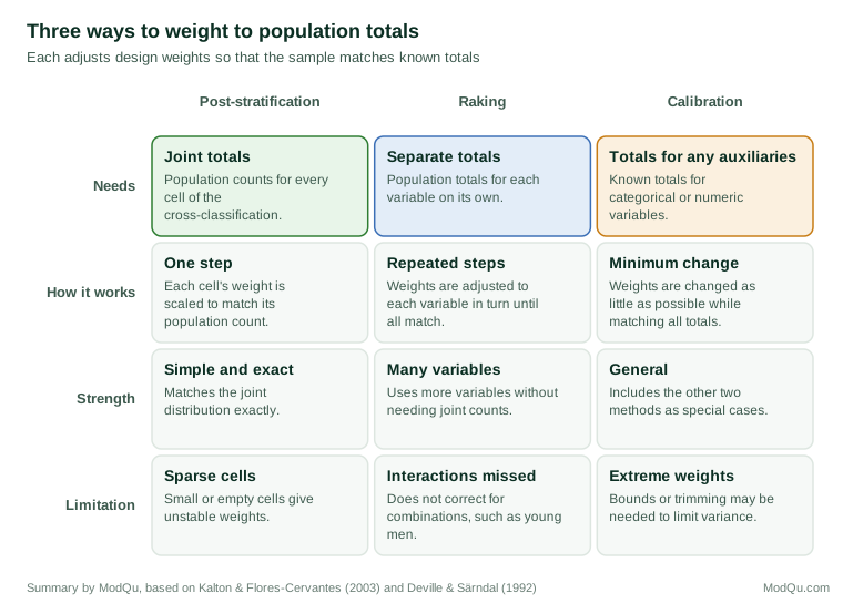
After nonresponse adjustment, the weighted sample may still differ from the population on characteristics such as age, sex, education or region, for which accurate totals are available from a census or administrative records. The final stage adjusts the weights so that weighted sample totals match these known totals. The three main methods are compared in Figure 1.
Post-stratification
Post-stratification divides the sample into cells defined by one or more variables, such as age group by sex, and scales the weights in each cell so that the weighted count equals the known population count for that cell (Holt & Smith, 1979). Figure 2 shows a simple example with three age groups.
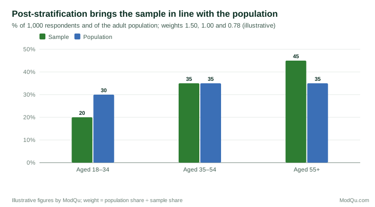
In the example, a survey of 1,000 adults has too few young respondents and too many older ones. Each respondent aged 18 to 34 receives a weight of 30 ÷ 20 = 1.50, each respondent aged 35 to 54 a weight of 1.00 and each respondent aged 55 and over a weight of 35 ÷ 45 = 0.78. Suppose 80 per cent of young respondents, 65 per cent of middle-aged respondents and 40 per cent of older respondents use online banking. The unweighted estimate is 56.8 per cent. The weighted estimate, which gives each age group its correct share, is 60.8 per cent (illustrative example).
Post-stratification is simple and matches the joint distribution of the chosen variables exactly. Its weakness is that the number of cells grows quickly as variables are added. With age, sex, region and education, there may be hundreds of cells, many with few or no respondents. Small cells produce unstable weights, and empty cells cannot be weighted at all. Cells are often combined, or collapsed, to avoid this problem (Kalton & Flores-Cervantes, 2003).
Raking
Raking, also called iterative proportional fitting, adjusts weights to match the totals of several variables one at a time, without needing their joint distribution. The weights are first adjusted to match the age distribution, then the sex distribution, then the region distribution and so on. Because each adjustment can disturb the match on earlier variables, the cycle is repeated until all totals match within a small tolerance (Deming & Stephan, 1940; Battaglia et al., 2009).
Raking allows many more variables to be used than post-stratification, because each needs only its own population totals. This is useful when joint totals are not published or when cells would be too sparse. Its limitation is that it matches only the separate distributions, not their combinations. If the sample has too few young men but the right number of young people and of men overall, raking on age and sex separately will not correct the shortage. Including important interactions, such as age by sex, as raking variables addresses this (Battaglia et al., 2009; Kolenikov, 2014).
Raking became a standard method in opinion polling and many other surveys. Analyses of polling errors in the 2016 United States election found that many polls had not weighted by education, although less educated voters were under-represented and voted differently from others. Adding education to the raking variables reduced the error (Kennedy et al., 2018).
Calibration
Calibration is a general framework that includes post-stratification and raking as special cases. Deville and Särndal (1992) defined calibration estimators as those that adjust design weights as little as possible, according to a chosen measure of distance, while making weighted totals of auxiliary variables equal to known population totals. Different distance measures give different methods: one gives the generalised regression estimator, another gives raking. Calibration can use categorical and numeric variables together, such as age groups and total income (Särndal et al., 1992; Särndal & Lundström, 2005).
A practical advantage of calibration is that bounds can be set on how much any weight can change. This prevents a few respondents from receiving very large or very small weights. Calibration can also be used to combine nonresponse adjustment and adjustment to population totals in a single step when the same variables serve both purposes (Särndal & Lundström, 2005; Haziza & Beaumont, 2017).
Trade-offs in weighting
Bias and variance
Weighting reduces bias when the weighting variables are related to both the reasons for nonresponse or undercoverage and the survey outcomes. It also increases variance, because unequal weights reduce the effective sample size. Kish (1992) gave a widely used approximation: the variance of an estimate is increased by a factor of about one plus the squared coefficient of variation of the weights. In the age example above, this factor is about 1.07, a modest loss. Weights that vary widely can increase variance much more.
Trimming
Very large weights give a few respondents great influence over the results. Trimming caps weights at a chosen maximum and redistributes the excess to other respondents. Trimming reduces variance but can reintroduce some bias, so the cap should be chosen with care (Potter, 1990; Valliant et al., 2018).
Choosing variables
The choice of weighting variables is the most important decision in weighting. Variables should be measured in the same way in the survey and in the source of population totals, should be related to response or coverage, and should be related to the survey's main measures (Brick, 2013). Mercer et al. (2018) compared weighting methods for online opt-in samples and found that the choice of variables mattered more than the statistical method: adding variables related to the outcomes, such as political engagement for political surveys, reduced bias more than switching between raking, matching and propensity methods.
Limits of weighting
Weighting can only correct for differences captured by the weighting variables. If respondents differ from nonrespondents in ways not related to those variables, bias remains. Weighting cannot create information about groups that are absent from the sample: if no respondents come from a group, no weight can represent it (Groves et al., 2009; Bethlehem, 2009).
Estimating precision with weights
Weights affect not only estimates but also their standard errors. Standard formulas that assume a simple random sample understate the uncertainty of weighted estimates, because they ignore the variation in weights and the effect of the adjustment steps. Survey software estimates variance using the design information, usually by linearisation or by replication methods such as the jackknife and bootstrap. Replication methods repeat the whole weighting process on many subsamples, so that the uncertainty introduced by nonresponse adjustment and calibration is captured (Valliant et al., 2018; Lohr, 2021). Publishing replicate weights with a dataset allows users to estimate standard errors correctly without access to confidential design details.
Weighting in business surveys
Business surveys raise particular weighting issues. Businesses vary enormously in size, so samples are usually stratified by size, with the largest businesses selected with certainty. Design weights then range from one for the largest firms to several hundred for the smallest. Calibration often uses numeric auxiliary variables such as employment or turnover from a business register, so that weighted totals match register totals. Because a single very large firm can dominate an industry total, outlier treatment and careful handling of nonresponse among large firms matter more than in household surveys. Register information is also often out of date, so businesses that have grown, shrunk or changed industry since the register was compiled need special treatment.
Weighting repeated and panel surveys
Surveys repeated over time, such as monthly or annual trackers, need weights that are consistent from one round to the next. Changing weighting variables or population sources between rounds can create apparent changes that reflect the method rather than the population. When population totals are updated, for example after a new census, many organisations revise past estimates so that the series remains comparable.
Panel surveys, which follow the same people over time, need additional adjustments for attrition. Each wave's weights are usually built from the previous wave's weights, adjusted for the people who drop out, using information collected from them in earlier waves. Because so much is known about those who leave a panel, attrition adjustments can be more effective than nonresponse adjustments in a cross-sectional survey.
Model-based alternatives
Some researchers combine weighting with statistical models. Multilevel regression and post-stratification fits a model that predicts the outcome for each population cell from the sample and then weights the predictions by the cell's population count. This allows estimates for small areas or groups where the sample is thin (Park et al., 2004). Gelman (2007) argued that model-based approaches can handle many weighting variables more stably than classical weighting, although they depend on the model being appropriate.
Good practice
Several practices improve the quality of weights:
- Begin with correct design weights and adjust for nonresponse before adjusting to population totals.
- Use population totals from reliable, recent sources that measure variables in the same way as the survey.
- Check cell sizes and collapse small cells before post-stratifying.
- Include important interactions when raking.
- Examine the distribution of weights and the design effect, and trim extreme weights if needed.
- Document the variables, sources and methods used, so users can judge the weights (Valliant et al., 2018).
Conclusion
Survey weights connect a sample to the population it represents. Design weights account for how the sample was selected, nonresponse adjustments account for who responded, and post-stratification, raking and calibration align the sample with known population totals. Each method has strengths and limits, and each involves a trade-off between reducing bias and increasing variance. The most important choices concern which variables to use and how to handle extreme weights. When made carefully, these choices allow survey results to describe the population, not just the people who happened to respond.
References
Battaglia, M. P., Izrael, D., Hoaglin, D. C., & Frankel, M. R. (2009). Practical considerations in raking survey data. Survey Practice, 2(5). https://doi.org/10.29115/SP-2009-0019
Bethlehem, J. (2009). Applied survey methods: A statistical perspective. Wiley. https://doi.org/10.1002/9780470494998
Brick, J. M. (2013). Unit nonresponse and weighting adjustments: A critical review. Journal of Official Statistics, 29(3), 329–353. https://doi.org/10.2478/jos-2013-0026
Deming, W. E., & Stephan, F. F. (1940). On a least squares adjustment of a sampled frequency table when the expected marginal totals are known. The Annals of Mathematical Statistics, 11(4), 427–444. https://doi.org/10.1214/aoms/1177731829
Deville, J.-C., & Särndal, C.-E. (1992). Calibration estimators in survey sampling. Journal of the American Statistical Association, 87(418), 376–382. https://doi.org/10.1080/01621459.1992.10475217
Gelman, A. (2007). Struggles with survey weighting and regression modeling. Statistical Science, 22(2), 153–164. https://doi.org/10.1214/088342306000000691
Groves, R. M., Fowler, F. J., Jr., Couper, M. P., Lepkowski, J. M., Singer, E., & Tourangeau, R. (2009). Survey methodology (2nd ed.). Wiley.
Haziza, D., & Beaumont, J.-F. (2017). Construction of weights in surveys: A review. Statistical Science, 32(2), 206–226. https://doi.org/10.1214/16-STS608
Holt, D., & Smith, T. M. F. (1979). Post stratification. Journal of the Royal Statistical Society: Series A (General), 142(1), 33–46. https://doi.org/10.2307/2344652
Kalton, G., & Flores-Cervantes, I. (2003). Weighting methods. Journal of Official Statistics, 19(2), 81–97.
Kennedy, C., Blumenthal, M., Clement, S., Clinton, J. D., Durand, C., Franklin, C., McGeeney, K., Miringoff, L., Olson, K., Rivers, D., Saad, L., Witt, G. E., & Wlezien, C. (2018). An evaluation of the 2016 election polls in the United States. Public Opinion Quarterly, 82(1), 1–33. https://doi.org/10.1093/poq/nfx047
Kish, L. (1992). Weighting for unequal P<sub>i</sub>. Journal of Official Statistics, 8(2), 183–200.
Kolenikov, S. (2014). Calibrating survey data using iterative proportional fitting (raking). The Stata Journal, 14(1), 22–59. https://doi.org/10.1177/1536867X1401400104
Little, R. J., & Vartivarian, S. (2005). Does weighting for nonresponse increase the variance of survey means? Survey Methodology, 31(2), 161–168.
Little, R. J. A. (1986). Survey nonresponse adjustments for estimates of means. International Statistical Review, 54(2), 139–157. https://doi.org/10.2307/1403140
Lohr, S. L. (2021). Sampling: Design and analysis (3rd ed.). CRC Press. https://doi.org/10.1201/9780429298899
Mercer, A., Lau, A., & Kennedy, C. (2018). For weighting online opt-in samples, what matters most? Pew Research Center.
Park, D. K., Gelman, A., & Bafumi, J. (2004). Bayesian multilevel estimation with poststratification: State-level estimates from national polls. Political Analysis, 12(4), 375–385. https://doi.org/10.1093/pan/mph024
Potter, F. J. (1990). A study of procedures to identify and trim extreme sampling weights. In Proceedings of the Survey Research Methods Section (pp. 225–230). American Statistical Association.
Särndal, C.-E., & Lundström, S. (2005). Estimation in surveys with nonresponse. Wiley. https://doi.org/10.1002/0470011351
Särndal, C.-E., Swensson, B., & Wretman, J. (1992). Model assisted survey sampling. Springer. https://doi.org/10.1007/978-1-4612-4378-6
Valliant, R., Dever, J. A., & Kreuter, F. (2018). Practical tools for designing and weighting survey samples (2nd ed.). Springer. https://doi.org/10.1007/978-3-319-93632-1