
Surveys · Nonresponse, weighting and data quality
Imputation of Missing Survey Data: Methods and Assumptions
When survey respondents skip questions, researchers can fill the gaps by imputation. This article explains the main imputation methods, from simple substitution to multiple imputation and machine learning, the assumptions each depends on and how to use and report imputed data responsibly.
Nearly every survey dataset has gaps. Respondents decline to give their income, do not know the value of their home, skip a question by mistake or stop before the end. These gaps are called item nonresponse. Analysts then face a choice: drop the respondents with missing answers, analyse only the answers that exist, or fill the gaps with plausible values. Filling the gaps is called imputation (Little & Rubin, 2019).
Imputation is widely used in official statistics, academic research and market research. It produces a complete dataset that is easy to analyse and can reduce bias when the missing answers differ from the reported ones. It also creates values that no respondent gave, and if it is done carelessly it can distort distributions, weaken relationships between variables and make estimates look more precise than they are (Rubin, 1987; Brick & Kalton, 1996). This article explains why imputation is used, the main methods, the assumptions behind them and how to use imputed data responsibly.
Why not simply drop missing cases?
The simplest approach to missing data is complete-case analysis: each analysis uses only respondents who answered every question involved. It is the default in many software packages. It has two drawbacks. First, it discards information. If a model uses ten variables, each missing for 5 per cent of respondents, up to 40 per cent of cases may be lost, even though most of those respondents answered most of the questions. Second, it can bias results. If people with high incomes are more likely to skip the income question, an analysis of those who answered will understate average income (Little & Rubin, 2019).
Another approach, available-case analysis, uses every answer available for each statistic, so that different statistics are based on different sets of respondents. This keeps more data but can produce results that do not fit together, such as correlations that are mathematically impossible when combined (Schafer & Graham, 2002).
Imputation addresses both problems by creating a complete dataset. Whether it reduces bias depends on how well the imputation method captures the relationship between the missing values and the information that is available.
Why answers are missing: three assumptions
The behaviour of any imputation method depends on why data are missing. Rubin (1976) defined three situations that remain the foundation of missing data theory (Little & Rubin, 2019).
Missing completely at random (MCAR). The chance that an answer is missing is unrelated to any characteristic of the respondent, observed or unobserved. A question accidentally left off some printed questionnaires is an example. Under MCAR, complete-case analysis is unbiased, though wasteful.
Missing at random (MAR). The chance that an answer is missing depends on characteristics that are observed, but not on the missing value itself once those characteristics are taken into account. For example, older respondents may be more likely to skip an income question, but among respondents of the same age, education and employment status, those who skip it have similar incomes to those who answer. Most imputation methods assume MAR.
Missing not at random (MNAR). The chance that an answer is missing depends on the missing value itself, even after accounting for observed characteristics. If people with very high incomes decline to report them, regardless of their age, job or education, income is MNAR. Imputation under the MAR assumption will then still understate high incomes.
The MAR assumption cannot be tested from the data alone, because it concerns values that were not observed. Researchers can make it more plausible by including in the imputation model variables that predict both the missing values and the likelihood of missingness. They can also test how sensitive their results are to departures from it (Schafer & Graham, 2002; van Buuren, 2018).
The main imputation methods
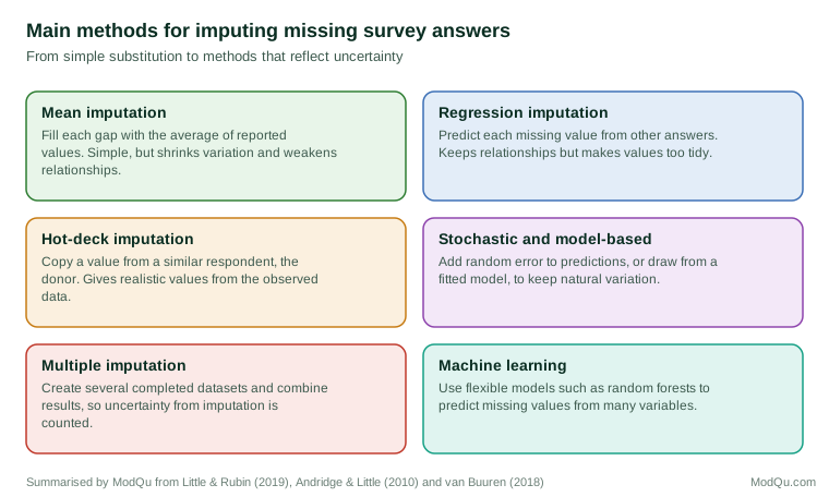
Figure 1 summarises the main families of imputation methods.
Mean imputation
Mean imputation replaces each missing value with the average of the reported values, sometimes within groups such as age bands. It is simple and preserves the overall mean if data are MCAR. It has serious drawbacks. Because every imputed value is the same, it shrinks the spread of the distribution, understates variance and weakens correlations with other variables. Estimates of the share of people above a threshold, such as those with incomes over a certain level, can be badly distorted (Little & Rubin, 2019). Mean imputation is rarely recommended except for minor variables with very little missing data.
Regression imputation
Regression imputation predicts each missing value from other answers using a model fitted to the respondents who answered. Income might be predicted from age, education, occupation, hours worked and region. This preserves relationships between the imputed variable and the predictors and can reduce bias under MAR. Its weakness is that predicted values lie exactly on the regression line, so they are less variable than real values. Correlations with the predictors are overstated, and the spread of the distribution is understated (Little, 1988).
Hot-deck imputation
Hot-deck imputation fills each missing value by copying the value from a similar respondent, called a donor. Donors are chosen from respondents who match the recipient on key characteristics, such as age group, sex and region, or who are closest according to a distance measure or a predicted value. Hot-deck methods have long been used in official statistics, including census and labour force surveys, because they produce realistic values, preserve the distribution of the variable and need no explicit model (Andridge & Little, 2010).
Andridge and Little (2010) reviewed hot-deck methods and identified several decisions that affect their performance: which variables define similarity, how donors are chosen within a group, whether the same donor can be used many times and how to estimate variance afterwards. Using a donor many times can reduce precision, and matching on too few variables can leave bias.
A variant used for numeric variables is predictive mean matching. A regression model predicts the value for each respondent and each nonrespondent, and each nonrespondent receives the actual value of a respondent whose prediction is close to theirs. This combines the strengths of regression and hot-deck methods: the model chooses donors, but the imputed values are real observed values (van Buuren, 2018).
Stochastic and model-based imputation
To restore natural variation, stochastic regression imputation adds a random error to each predicted value, drawn from the distribution of residuals in the fitted model. More generally, model-based imputation draws each missing value from a probability distribution estimated from the data. Joint models, such as the multivariate normal model, impute several variables at once (Schafer, 1997). These methods preserve variances and relationships better than deterministic methods but depend on the model being appropriate.
When many variables have missing values, specifying a single joint model is difficult. Sequential regression or chained equations imputation handles this by fitting a separate model for each variable with missing values, conditional on all the others, and cycling through them repeatedly. Each variable can have its own type of model, such as linear regression for income and logistic regression for employment status. Raghunathan et al. (2001) developed this approach for large surveys, and van Buuren and Groothuis-Oudshoorn (2011) implemented it in widely used software. White et al. (2011) provided practical guidance on its use.
Machine learning methods
Flexible machine learning models, such as classification and regression trees and random forests, can be used to predict missing values. They can capture complex interactions and non-linear relationships without the analyst specifying them in advance. Stekhoven and Bühlmann (2012) described a random forest method that imputes mixed numeric and categorical data. Such methods are useful when there are many potential predictors, but they can be harder to explain and, like other single imputation methods, do not by themselves reflect the uncertainty of imputed values.
Imputation and uncertainty
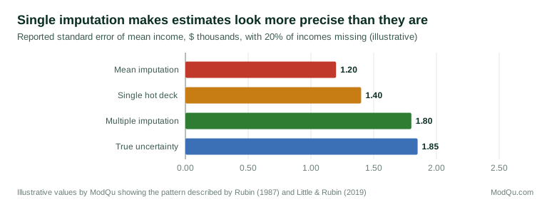
Any single imputation, however good, treats imputed values as if they had been observed. Standard errors calculated from the completed dataset are then too small, because they ignore the uncertainty about what the missing values really were. Confidence intervals are too narrow and significance tests too optimistic (Rubin, 1987). Figure 2 illustrates the problem.
Multiple imputation
Multiple imputation, proposed by Rubin (1987), addresses this problem. Instead of filling each gap once, the analyst creates several completed datasets, each with different imputed values drawn from their predicted distribution. The analysis is run separately on each dataset, and the results are combined using simple rules. The combined estimate is the average across datasets. Its variance has two parts: the average variance within datasets and the variance between datasets. The between-dataset variance reflects the uncertainty caused by the missing data (Rubin, 1987, 1996).
Early guidance suggested that three to five imputations were enough. Later work showed that more imputations, often 20 or more, are needed for stable standard errors and significance tests when much information is missing (Graham et al., 2007; White et al., 2011).
Multiple imputation has become a standard tool in many fields. Schenker et al. (2006) described its use for missing income data in a major national health survey, where income was multiply imputed using a sequence of regression models and released to users as several completed datasets. Sterne et al. (2009) set out its potential and pitfalls in medical research, emphasising that the imputation model must include the variables used in the analysis, including the outcome.
Variance estimation for single imputation
Some statistical agencies prefer single imputation, because it produces one dataset that is simpler to release and use. In that case, special variance estimation methods can account for imputation. Rao and Shao (1992) developed a jackknife method that adjusts imputed values in each replicate, giving approximately correct standard errors under hot-deck imputation. Fay (1996) and Haziza (2009) discussed different frameworks for inference with imputed survey data. These methods require information about which values were imputed and how.
Choosing variables for the imputation model
The imputation model should include:
- variables that predict the missing values;
- variables that predict whether values are missing, which makes the MAR assumption more plausible;
- all variables that will be used in later analyses, including outcomes; and
- design features, such as strata, clusters and weights, or variables closely related to them.
Leaving a variable out of the imputation model implicitly assumes it is unrelated to the imputed variable among nonrespondents, which weakens its relationships in the completed data. Meng (1994) described the problems that arise when the imputer's model and the analyst's model differ, a situation he called uncongeniality. Including more variables in the imputation model than in any one analysis is generally safer than including fewer (Schafer & Graham, 2002; van Buuren, 2018).
Editing, deductive imputation and business surveys
Edits and deductive imputation
Imputation in official statistics is closely linked to editing, the process of checking answers against rules. Some answers are not missing but impossible or inconsistent, such as a child listed as older than their parent, or component costs that add to more than the reported total. Fellegi and Holt (1976) proposed a systematic approach in which the smallest possible number of fields is changed so that a record passes all edit rules, and the changed fields are then imputed. Their framework remains the basis of automated edit and imputation systems in many statistical agencies.
Sometimes a missing value can be worked out exactly from other answers. If a respondent reports total household income and every component except one, the missing component can be calculated. If a person reports being retired and gives no hours of work, zero hours can be filled in. This is called deductive or logical imputation. It should be applied before any statistical method, because it uses information that is certain rather than predicted (Kalton & Kasprzyk, 1986).
Business surveys
Business and establishment surveys often use methods suited to their data. Businesses vary greatly in size, and their values are strongly related to known size measures, such as employment or turnover on a business register. Ratio imputation predicts a missing value by multiplying the business's size measure by the ratio observed among similar responding businesses. In repeated surveys, the business's own previous report, adjusted by the change observed among similar businesses, is usually the best predictor of its current value. Because a few large businesses can account for much of an industry's total, statistical agencies often contact large nonresponding businesses again or use administrative data rather than impute them (Kalton & Kasprzyk, 1986; Haziza, 2009).
Imputation in practice
Using partial information
Many surveys collect partial information that improves imputation. When respondents decline to give an exact income, follow-up bracket questions, such as "Is it more than $50,000?", often recover a range. Imputation can then draw values within the reported range, greatly reducing error (Juster & Smith, 1997). Previous waves of a panel survey, administrative records and answers to related questions, such as sources of income, provide further information.
Checking imputations
Imputed values should be checked. Analysts can compare the distributions of imputed and reported values, check that imputed values respect logical constraints, such as no negative ages and no retired people with full-time hours, and examine whether key relationships look plausible. Differences between imputed and observed distributions are expected under MAR when missingness depends on observed variables, but large or unexplained differences suggest problems with the model (van Buuren, 2018).
Flagging imputed values
Imputed values should always be flagged in released data, so that users can identify them, compare results with and without them and choose their own approach. Documentation should state which variables were imputed, how much was imputed, the method used and the variables in the model (Brick & Kalton, 1996).
When the share of missing data is large
Imputation works best when a modest share of values is missing and good predictors are available. When a large share is missing, results depend heavily on the imputation model, and conclusions should be presented with caution. For variables known to be affected by MNAR, such as very high incomes, sensitivity analyses can show how results would change if nonrespondents differed systematically from similar respondents (Little & Rubin, 2019). A common form of sensitivity analysis shifts the imputed values by a fixed amount, for example assuming that nonrespondents' incomes are 5, 10 or 20 per cent higher than those of similar respondents, and shows how the main estimates change. If conclusions hold across a plausible range of shifts, users can have more confidence in them; if they change sharply, the uncertainty should be reported (van Buuren, 2018). Moore et al. (2000) noted that income questions are especially prone to both nonresponse and reporting error, so imputation of income should be considered together with measurement quality.
An example
A household survey of 4,000 respondents asks about income, housing costs, employment and health. Exact household income is missing for 18 per cent of respondents, although two thirds of these answered follow-up bracket questions. Housing costs are missing for 7 per cent and several health items for 2 to 4 per cent.
The survey team uses chained equations imputation with predictive mean matching for numeric variables and logistic models for categorical ones. The imputation model includes all survey variables used in published tables, the bracket information, region, household size, tenure and the survey weights. It creates 20 completed datasets. For the main publication, results are combined across the 20 datasets, and standard errors include the between-imputation variance. Mean household income in the combined results is 5 per cent higher than among respondents who reported an exact amount, consistent with higher-income households being more likely to decline the exact question. The released data file includes flags for all imputed values and the 20 imputations, with guidance for users (illustrative example).
Common mistakes
Several mistakes are common in practice (Schafer & Graham, 2002; Sterne et al., 2009):
- Using mean imputation for important variables, which distorts distributions and relationships.
- Treating single imputed values as observed, which understates standard errors.
- Leaving the outcome out of the imputation model, which weakens estimated relationships towards zero.
- Imputing without flags, so that users cannot tell which values were reported.
- Ignoring logical constraints, producing impossible combinations of answers.
- Assuming MAR without thought, when there are reasons to believe missingness depends on the missing values themselves.
Conclusion
Imputation fills gaps in survey data so that analyses can use all available information. Simple methods, such as mean imputation, are easy but distort results. Regression, hot-deck and model-based methods preserve more of the structure of the data, and multiple imputation adds a way to reflect the uncertainty that imputation introduces. All methods rest on assumptions about why data are missing, most commonly that missingness can be explained by observed variables. Choosing good predictors, using partial information, checking imputations, flagging imputed values and reporting methods clearly make imputation a sound part of producing survey knowledge.
References
Andridge, R. R., & Little, R. J. A. (2010). A review of hot deck imputation for survey non-response. International Statistical Review, 78(1), 40–64. https://doi.org/10.1111/j.1751-5823.2010.00103.x
Brick, J. M., & Kalton, G. (1996). Handling missing data in survey research. Statistical Methods in Medical Research, 5(3), 215–238. https://doi.org/10.1177/096228029600500302
Fay, R. E. (1996). Alternative paradigms for the analysis of imputed survey data. Journal of the American Statistical Association, 91(434), 490–498. https://doi.org/10.1080/01621459.1996.10476909
Fellegi, I. P., & Holt, D. (1976). A systematic approach to automatic edit and imputation. Journal of the American Statistical Association, 71(353), 17–35. https://doi.org/10.1080/01621459.1976.10481472
Graham, J. W., Olchowski, A. E., & Gilreath, T. D. (2007). How many imputations are really needed? Some practical clarifications of multiple imputation theory. Prevention Science, 8(3), 206–213. https://doi.org/10.1007/s11121-007-0070-9
Haziza, D. (2009). Imputation and inference in the presence of missing data. In D. Pfeffermann & C. R. Rao (Eds.), Handbook of statistics: Vol. 29A. Sample surveys: Design, methods and applications (pp. 215–246). Elsevier. https://doi.org/10.1016/S0169-7161(08)00010-0
Juster, F. T., & Smith, J. P. (1997). Improving the quality of economic data: Lessons from the HRS and AHEAD. Journal of the American Statistical Association, 92(440), 1268–1278. https://doi.org/10.1080/01621459.1997.10473648
Kalton, G., & Kasprzyk, D. (1986). The treatment of missing survey data. Survey Methodology, 12(1), 1–16.
Little, R. J. A., & Rubin, D. B. (2019). Statistical analysis with missing data (3rd ed.). Wiley. https://doi.org/10.1002/9781119482260
Little, R. J. A. (1988). Missing-data adjustments in large surveys. Journal of Business & Economic Statistics, 6(3), 287–296. https://doi.org/10.1080/07350015.1988.10509663
Meng, X.-L. (1994). Multiple-imputation inferences with uncongenial sources of input. Statistical Science, 9(4), 538–558. https://doi.org/10.1214/ss/1177010269
Moore, J. C., Stinson, L. L., & Welniak, E. J., Jr. (2000). Income measurement error in surveys: A review. Journal of Official Statistics, 16(4), 331–361.
Raghunathan, T. E., Lepkowski, J. M., Van Hoewyk, J., & Solenberger, P. (2001). A multivariate technique for multiply imputing missing values using a sequence of regression models. Survey Methodology, 27(1), 85–95.
Rao, J. N. K., & Shao, J. (1992). Jackknife variance estimation with survey data under hot deck imputation. Biometrika, 79(4), 811–822. https://doi.org/10.1093/biomet/79.4.811
Rubin, D. B. (1976). Inference and missing data. Biometrika, 63(3), 581–592. https://doi.org/10.1093/biomet/63.3.581
Rubin, D. B. (1987). Multiple imputation for nonresponse in surveys. Wiley. https://doi.org/10.1002/9780470316696
Rubin, D. B. (1996). Multiple imputation after 18+ years. Journal of the American Statistical Association, 91(434), 473–489. https://doi.org/10.1080/01621459.1996.10476908
Schafer, J. L., & Graham, J. W. (2002). Missing data: Our view of the state of the art. Psychological Methods, 7(2), 147–177. https://doi.org/10.1037/1082-989X.7.2.147
Schafer, J. L. (1997). Analysis of incomplete multivariate data. Chapman & Hall.
Schenker, N., Raghunathan, T. E., Chiu, P.-L., Makuc, D. M., Zhang, G., & Cohen, A. J. (2006). Multiple imputation of missing income data in the National Health Interview Survey. Journal of the American Statistical Association, 101(475), 924–933. https://doi.org/10.1198/016214505000001375
Stekhoven, D. J., & Bühlmann, P. (2012). MissForest—Non-parametric missing value imputation for mixed-type data. Bioinformatics, 28(1), 112–118. https://doi.org/10.1093/bioinformatics/btr597
Sterne, J. A. C., White, I. R., Carlin, J. B., Spratt, M., Royston, P., Kenward, M. G., Wood, A. M., & Carpenter, J. R. (2009). Multiple imputation for missing data in epidemiological and clinical research: Potential and pitfalls. BMJ, 338, b2393. https://doi.org/10.1136/bmj.b2393
van Buuren, S., & Groothuis-Oudshoorn, K. (2011). mice: Multivariate imputation by chained equations in R. Journal of Statistical Software, 45(3), 1–67. https://doi.org/10.18637/jss.v045.i03
van Buuren, S. (2018). Flexible imputation of missing data (2nd ed.). CRC Press. https://doi.org/10.1201/9780429492259
White, I. R., Royston, P., & Wood, A. M. (2011). Multiple imputation using chained equations: Issues and guidance for practice. Statistics in Medicine, 30(4), 377–399. https://doi.org/10.1002/sim.4067