
Statistics · Foundations
The Central Limit Theorem Explained
What the central limit theorem says, why it lets analysts put margins of error on averages from skewed data, how large a sample really needs to be, and when the theorem fails.
Almost every margin of error, confidence interval and significance test reported from a survey rests on one result: the central limit theorem. It explains why the average of a sample behaves in a predictable way even when the individual answers do not. Customer spending, household income, time on a website and the number of products bought are all lopsided, with many small values and a few very large ones. Yet the average of a reasonably large sample from any of them follows a familiar bell-shaped curve, and that curve tells us how far the sample average is likely to be from the true population value.
What the theorem says
Imagine drawing a random sample of n customers from a large population and calculating their average monthly spend. Draw another sample of the same size and the average will be a little different. If this were repeated thousands of times, the averages would form a distribution of their own, called the sampling distribution of the mean. The central limit theorem describes the shape of that distribution.
In its classical form, the theorem says that if observations are independent, come from the same distribution, and that distribution has a finite mean μ and a finite standard deviation σ, then as the sample size grows the distribution of the sample mean approaches a normal distribution with mean μ and standard deviation σ ÷ √n (Wasserman, 2004). Written as a standardised quantity:
Z = (x̄ − μ) ÷ (σ ÷ √n) → N(0, 1) as n → ∞
Three features of this statement deserve emphasis.
- It is about averages, not individual values. The theorem does not say that the data become normal. Spending by individual customers stays as skewed as it ever was. Only the distribution of the average across many hypothetical samples approaches the bell shape.
- The starting shape barely matters. The population can be skewed, lumpy or even a simple yes/no variable. As long as its variance is finite, averages of large samples will be close to normal. This is what makes the theorem so useful.
- It is a statement about a limit. Strictly, the theorem describes what happens as n grows without bound. For any real sample it is an approximation, and how good that approximation is depends on the sample size and on the shape of the population.
Because a proportion is simply the average of a variable coded 1 for "yes" and 0 for "no", the theorem covers survey percentages as well as averages of numeric answers.
A short history
The theorem took nearly two centuries to reach its modern form. Abraham de Moivre showed in the 1730s that the number of heads in many coin tosses could be approximated by a bell-shaped curve, and Pierre-Simon Laplace extended the idea to sums of more general errors in the early nineteenth century. Russian mathematicians, Aleksandr Lyapunov in particular, gave the first general proofs around 1900, and Lindeberg (1922) established a set of conditions under which sums of independent variables that need not share the same distribution still tend to normality. The name itself is usually credited to George Pólya, who in 1920 called it "central" because of its central place in probability theory (Le Cam, 1986). Fischer (2011) traces this development in detail.
Two later contributions matter for applied work. Berry (1941), and independently Carl-Gustav Esseen, put a bound on how quickly the approximation improves as the sample grows, which turns a statement about infinity into one about real sample sizes. And Student (1908) worked out the t distribution, which handles the fact that in practice σ is unknown and must be estimated from the same sample.
Seeing the theorem at work
The easiest way to understand the theorem is to watch it happen. Figure 1 starts with a hypothetical population of customer spend that is strongly right-skewed: most customers spend a little, a few spend a lot, and the average is $60. The top-left panel shows this population. The other panels show the exact distribution of the average spend for random samples of 2, 5 and 30 customers, with the normal curve predicted by the theorem drawn over each.
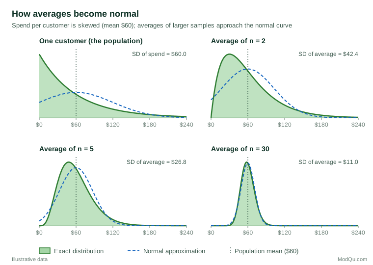
Two things happen as the sample grows. First, the shape changes: the skew is pulled in and the distribution becomes more symmetrical, until at n = 30 the exact curve and the normal curve are hard to tell apart. Second, the spread shrinks. The standard deviation of the average falls in proportion to 1 ÷ √n, from $60 for a single customer to about $11 for an average of 30. The theorem adds the shape, which lets us turn a standard deviation into a probability statement.
Why it matters: standard errors and confidence intervals
The standard deviation of the sampling distribution is called the standard error (SE). For a mean it is estimated from the sample standard deviation s:
SE(x̄) = s ÷ √n
For a proportion p it is:
SE(p) = √( p(1 − p) ÷ n )
Because the sampling distribution is approximately normal, about 95% of sample means fall within 1.96 standard errors of the population mean. Turning this around gives the familiar 95% confidence interval:
x̄ ± 1.96 × SE
Without the central limit theorem we would need to know the exact shape of the population before we could attach a margin of error to its average. With it, one formula serves for spending, satisfaction scores, purchase counts and percentages alike. The same logic underlies the z and t tests, the standard errors printed by regression software and the significance tests used to read A/B experiments (Kohavi et al., 2020).
A worked example
Suppose a hypothetical survey of 400 randomly selected customers of an online retailer finds that average spend in the past month was $62, with a standard deviation of $85. The standard deviation is larger than the mean, a clear sign of a skewed distribution: many customers spent little and a few spent several hundred dollars.
The standard error of the mean is:
SE = 85 ÷ √400 = 85 ÷ 20 = 4.25
and the 95% confidence interval is:
62 ± 1.96 × 4.25 = 62 ± 8.33, or $53.67 to $70.33
None of the individual spending figures needs to be normally distributed for this calculation to be reasonable. What matters is that the sample average of 400 customers has an approximately normal sampling distribution.
The same survey finds that 30% of customers would recommend the retailer to a friend. The standard error of this proportion is √(0.30 × 0.70 ÷ 400) ≈ 0.023, or 2.3 percentage points, giving a 95% interval of roughly 25.5% to 34.5%. This is the "margin of error of ±4.5 points" that would appear in a report.
Both calculations assume a simple random sample. As discussed below, weighting, clustering and non-response all change the picture.
How large is "large enough"?
Introductory courses often teach that the theorem "kicks in" at n = 30. That rule of thumb is convenient but has no general basis. The sample size needed depends mainly on how skewed and how heavy-tailed the population is. For a symmetrical population, a handful of observations may be enough. For a highly skewed one, hundreds or thousands may be needed.
The Berry–Esseen theorem makes this precise. It bounds the largest gap between the true distribution of the standardised mean, Fn, and the normal distribution, Φ:
max |Fn(x) − Φ(x)| ≤ C × ρ ÷ (σ3 × √n)
where ρ is the average absolute cubed deviation from the mean and C is a fixed constant (Berry, 1941; Durrett, 2019). The ratio ρ ÷ σ3 grows with skewness and with the weight of the tails, and the error shrinks only with √n. Quadrupling the sample halves the worst-case error. Higher-order (Edgeworth) expansions show that for the mean, the leading term of the error is driven by the population's skewness (Hall, 1992).
What this means for real confidence intervals is shown in Figure 2. For three hypothetical populations, 20,000 samples were simulated at each sample size, and the share of 95% t intervals that contained the true mean was recorded.
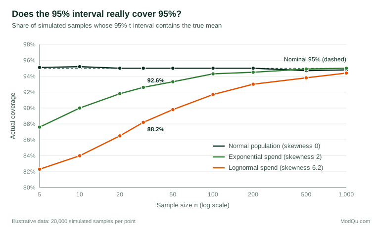
For the normal population the interval does exactly what it claims at every sample size. For exponential spending, with skewness of 2, coverage at n = 30 is about 93%, and the shortfall persists into the hundreds. For a more skewed lognormal population, coverage at n = 30 is only 88%: about one interval in eight misses the true mean instead of one in twenty. Boos and Hughes-Oliver (2000) reach the same conclusion analytically: the accuracy of z and t intervals depends chiefly on population skewness, and the errors are not symmetrical. With right-skewed data, intervals miss more often on one side than the other, which matters for one-sided tests.
Several practical rules follow from this work. Kohavi et al. (2014), drawing on large-scale online experiments, recommend a minimum of 355 × s2 independent observations per group when the absolute skewness s exceeds 1. For the exponential population above that is about 1,400; for the lognormal it is about 13,600. Johnson (1978) proposed a modified t interval that corrects for skewness, and resampling methods offer a more general check.
None of this means the theorem is fragile. Lumley et al. (2002) showed by simulation that t tests and linear regression remained valid for highly non-normal health cost data in large samples, and argued that the widespread belief that these methods require normal data is mistaken. Sawilowsky and Blair (1992) similarly found the t test fairly robust for many realistic non-normal distributions with moderate, equal group sizes, while noting weaknesses with small samples, one-tailed tests and extreme skew. The lesson is to match the sample size to the shape of the data, not to a single magic number.
When the theorem does not apply
The theorem has conditions, and real data sometimes break them.
Infinite or very large variance
The theorem requires a finite variance. Some distributions do not have one. The standard textbook example is the Cauchy distribution: the average of any number of Cauchy observations has exactly the same distribution as a single observation, so taking larger samples does not help at all (Durrett, 2019). Mandelbrot (1963) found that changes in commodity prices had tails so heavy that their variance appeared to be infinite, which undermined standard models built on the normal curve. Some business variables, such as revenue where a few clients account for most sales, behave in practice almost as badly, and a single extreme value can dominate the mean.
Dependent observations
The classical theorem assumes independent observations. Respondents interviewed in the same household, store or neighbourhood tend to be more alike than people chosen at random, and repeated measurements over time are often correlated. Ignoring clustering typically makes standard errors too small and intervals too narrow (Lumley, 2010).
Finite populations and complex designs
Survey samples are drawn without replacement from finite populations, often with stratification, clustering and unequal weights. Central limit theorems have been established for these designs too, and they justify the normal-based confidence intervals produced by survey software (Fuller, 2009). However, the relevant standard error is the design-based one, not s ÷ √n, and the effective sample size after weighting can be much smaller than the number of completed interviews (Lohr, 2021).
Statistics other than means
The theorem applies directly to means, proportions and sums, and through extensions to many smooth functions of them, such as regression coefficients. It does not guarantee normality for statistics such as the maximum, extreme percentiles, or ratios with a small denominator. For these, and for any statistic whose sampling distribution is in doubt, the bootstrap offers an alternative: resample the observed data many times, recompute the statistic, and look directly at its distribution (Efron, 1979; Efron & Tibshirani, 1994). Hesterberg (2015) recommends the bootstrap partly as a way to see how far a sampling distribution is from normal, which makes it a useful check on the theorem for skewed data.
Bias
Finally, the theorem says nothing about bias. It describes how a sample mean varies around the mean of the population that was actually sampled. If the sample frame misses some customers, or some groups are less likely to respond, the mean will be centred on the wrong value, and a large sample will simply produce a narrow interval around that wrong value. Margins of error based on the theorem describe random sampling error only.
Practical guidance for survey and business data
- Look at the data first. A histogram and a few summary statistics (mean versus median, skewness, the largest values) show whether a variable is close to symmetrical or has a long tail. Real data are rarely normal. Micceri (1989) examined 440 large-sample distributions of achievement and psychometric measures and found that none could be considered normal, which is why the theorem, rather than the data, carries most of the weight in practice.
- Match the sample size to the skewness. For roughly symmetrical rating scales and for proportions not too close to 0% or 100%, a few hundred respondents per group is usually ample. For spending, revenue and counts with long tails, check the skewness and consider rules such as 355 × s2 (Kohavi et al., 2014).
- Take care with proportions near 0% or 100%. The simple interval p ± 1.96 × SE can perform poorly when the proportion is small, even with large samples. Brown et al. (2001) document its erratic coverage and recommend alternatives such as the Wilson interval, and Agresti and Coull (1998) show that a simple adjustment (adding two successes and two failures) gives much better results.
- Report the median as well as the mean for skewed variables. The median describes the typical customer.
- Consider trimming, capping or transforming extreme values, and state clearly what was done. Wilcox (1998) shows that heavy tails and outliers can severely reduce the power of methods based on means, and that robust alternatives such as trimmed means often detect real differences that ordinary t tests miss.
- Use design-based standard errors for weighted or clustered samples, so that the interval reflects how the data were actually collected (Lohr, 2021; Lumley, 2010).
- Check doubtful cases with the bootstrap or simulation. If the result matters and the data are unusual, a resampling check is quick and shows whether the normal approximation is adequate (Efron & Tibshirani, 1994).
Common mistakes
- Believing the data must be normal. The theorem applies to the sampling distribution of the average. Skewed individual responses are not a reason to abandon a sound analysis.
- Treating n = 30 as a guarantee. As Figure 2 shows, intervals can fall well short of their stated confidence at n = 30, and even at several hundred, when the data are skewed.
- Applying the theorem to subgroups without checking their size. A survey of 2,000 may have only 40 respondents in a regional or demographic subgroup, and the subgroup's margin of error is governed by those 40.
- Ignoring dependence and design. Clustered, weighted and repeated-measures data need standard errors that reflect the design.
- Confusing precision with accuracy. A narrow interval from a large but biased sample is precisely wrong. The theorem controls random error, not selection or measurement error.
Key takeaways
The central limit theorem says that averages of independent observations from a population with finite variance have an approximately normal sampling distribution, centred on the population mean, with a standard deviation of σ ÷ √n. That single result justifies the standard error, the margin of error and most everyday tests applied to survey and business data, whatever the shape of the underlying responses.
The approximation improves only slowly, and the sample needed grows with skewness and heavy tails. It fails with infinite variance and says nothing about bias. Look at the data, size the sample to its shape, use design-based standard errors and check doubtful cases by resampling.
References
Agresti, A., & Coull, B. A. (1998). Approximate is better than "exact" for interval estimation of binomial proportions. The American Statistician, 52(2), 119–126. https://doi.org/10.1080/00031305.1998.10480550
Berry, A. C. (1941). The accuracy of the Gaussian approximation to the sum of independent variates. Transactions of the American Mathematical Society, 49(1), 122–136. https://doi.org/10.1090/S0002-9947-1941-0003498-3
Boos, D. D., & Hughes-Oliver, J. M. (2000). How large does n have to be for Z and t intervals? The American Statistician, 54(2), 121–128. https://doi.org/10.1080/00031305.2000.10474524
Brown, L. D., Cai, T. T., & DasGupta, A. (2001). Interval estimation for a binomial proportion. Statistical Science, 16(2), 101–133. https://doi.org/10.1214/ss/1009213286
Durrett, R. (2019). Probability: Theory and examples (5th ed.). Cambridge University Press. https://doi.org/10.1017/9781108591034
Efron, B. (1979). Bootstrap methods: Another look at the jackknife. The Annals of Statistics, 7(1), 1–26. https://doi.org/10.1214/aos/1176344552
Efron, B., & Tibshirani, R. J. (1994). An introduction to the bootstrap. Chapman and Hall/CRC. https://doi.org/10.1201/9780429246593
Fischer, H. (2011). A history of the central limit theorem: From classical to modern probability theory. Springer. https://doi.org/10.1007/978-0-387-87857-7
Fuller, W. A. (2009). Sampling statistics. Wiley. https://doi.org/10.1002/9780470523551
Hall, P. (1992). The bootstrap and Edgeworth expansion. Springer. https://doi.org/10.1007/978-1-4612-4384-7
Hesterberg, T. C. (2015). What teachers should know about the bootstrap: Resampling in the undergraduate statistics curriculum. The American Statistician, 69(4), 371–386. https://doi.org/10.1080/00031305.2015.1089789
Johnson, N. J. (1978). Modified t tests and confidence intervals for asymmetrical populations. Journal of the American Statistical Association, 73(363), 536–544. https://doi.org/10.1080/01621459.1978.10480051
Kohavi, R., Deng, A., Longbotham, R., & Xu, Y. (2014). Seven rules of thumb for web site experimenters. In Proceedings of the 20th ACM SIGKDD International Conference on Knowledge Discovery and Data Mining (pp. 1857–1866). ACM. https://doi.org/10.1145/2623330.2623341
Kohavi, R., Tang, D., & Xu, Y. (2020). Trustworthy online controlled experiments: A practical guide to A/B testing. Cambridge University Press. https://doi.org/10.1017/9781108653985
Le Cam, L. (1986). The central limit theorem around 1935. Statistical Science, 1(1), 78–91. https://doi.org/10.1214/ss/1177013818
Lindeberg, J. W. (1922). Eine neue Herleitung des Exponentialgesetzes in der Wahrscheinlichkeitsrechnung. Mathematische Zeitschrift, 15(1), 211–225. https://doi.org/10.1007/BF01494395
Lohr, S. L. (2021). Sampling: Design and analysis (3rd ed.). Chapman and Hall/CRC. https://doi.org/10.1201/9780429298899
Lumley, T. (2010). Complex surveys: A guide to analysis using R. Wiley. https://doi.org/10.1002/9780470580066
Lumley, T., Diehr, P., Emerson, S., & Chen, L. (2002). The importance of the normality assumption in large public health data sets. Annual Review of Public Health, 23(1), 151–169. https://doi.org/10.1146/annurev.publhealth.23.100901.140546
Mandelbrot, B. (1963). The variation of certain speculative prices. The Journal of Business, 36(4), 394–419. https://doi.org/10.1086/294632
Micceri, T. (1989). The unicorn, the normal curve, and other improbable creatures. Psychological Bulletin, 105(1), 156–166. https://doi.org/10.1037/0033-2909.105.1.156
Sawilowsky, S. S., & Blair, R. C. (1992). A more realistic look at the robustness and Type II error properties of the t test to departures from population normality. Psychological Bulletin, 111(2), 352–360. https://doi.org/10.1037/0033-2909.111.2.352
Student. (1908). The probable error of a mean. Biometrika, 6(1), 1–25. https://doi.org/10.1093/biomet/6.1.1
Wasserman, L. (2004). All of statistics: A concise course in statistical inference. Springer. https://doi.org/10.1007/978-0-387-21736-9
Wilcox, R. R. (1998). How many discoveries have been lost by ignoring modern statistical methods? American Psychologist, 53(3), 300–314. https://doi.org/10.1037/0003-066X.53.3.300