
Statistics · Foundations
Levels of Measurement: Nominal, Ordinal, Interval and Ratio
What the four levels of measurement mean, which summaries and tests suit each one, and how to handle rating scales and other awkward survey variables without misleading anyone.
Every survey dataset mixes different kinds of numbers. A respondent's region might be stored as 3, their satisfaction rating as 4, their age as 42 and their monthly spend as 180. All four are digits in a spreadsheet, but they do not carry the same information. Adding two region codes is meaningless, while adding two spending figures gives a useful total. The idea of levels of measurement describes these differences. It tells analysts which comparisons a set of numbers can support, which summaries are sensible and which conclusions would be misleading.
The standard classification was proposed by the psychologist S. S. Stevens, who divided measurement into four scales: nominal, ordinal, interval and ratio (Stevens, 1946). It is still taught everywhere, and it has also attracted sustained criticism. This article explains the four levels, applies them to survey and business data, and shows where the scheme should guide judgement rather than replace it.
Stevens's four scales
Stevens (1946) defined each scale by the transformations that leave its information unchanged. The fewer transformations a scale allows, the more it says.
Nominal
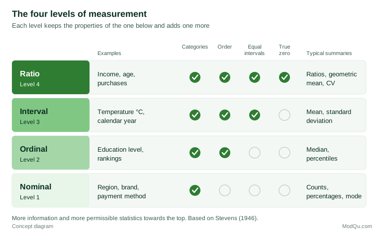
A nominal variable sorts cases into categories that have no natural order. Region, brand, payment method and yes/no answers are nominal. Numbers may be attached as labels (1 = North, 2 = South), but any other set of distinct labels would serve just as well. Sensible summaries are counts, percentages and the mode, the most common category.
Ordinal
An ordinal variable has categories with a meaningful order but unknown distances between them. Education level, brand rankings and the options "never, sometimes, often, always" are ordinal. We know that "often" is more than "sometimes", but not whether the step from "sometimes" to "often" is the same size as the step from "never" to "sometimes". Any transformation that keeps the order intact is permitted. Medians, percentiles and rank-based statistics are appropriate.
Interval
An interval variable has equal distances between values, so differences are meaningful, but its zero point is arbitrary. Temperature in degrees Celsius is the standard example: the difference between 10 °C and 20 °C equals the difference between 20 °C and 30 °C, but 0 °C does not mean "no temperature". Interval scales can be changed by any linear transformation (multiplying by a constant and adding another), which is how Celsius converts to Fahrenheit. Means, standard deviations and correlations are meaningful.
Ratio
A ratio variable has equal intervals and a true zero that means "none of the quantity". Income, age, number of purchases and time on a website are ratio measures. Because zero is real, ratios are meaningful: a customer who spends $200 has spent twice as much as one who spends $100. The only permitted transformation is multiplication by a positive constant, such as converting dollars to cents. All the statistics available at lower levels can be used, along with ratio-based summaries such as the coefficient of variation and the geometric mean.
The scales are cumulative. Each level keeps all the properties of the one below and adds one more, as Figure 1 shows.
Why the level matters
The level of measurement determines which statements about the data stay true when the numbers are relabelled in an allowed way. This is the idea of meaningfulness in measurement theory. A statement is meaningful if its truth does not depend on an arbitrary choice of scale (Hand, 1996).
Temperature shows the point clearly. On a day when it is 20 °C, it is tempting to say it is "twice as warm" as a 10 °C day. Converted to Fahrenheit, the same days are 68 °F and 50 °F, a ratio of 1.36 rather than 2. In kelvin, which has a true zero, the ratio is 293.15 ÷ 283.15, or about 1.04. The claim "twice as warm" depends on the scale chosen, so it is not meaningful, whereas statements about equal differences survive any change from Celsius to Fahrenheit.
Survey data contain the same traps in less obvious forms. If income is collected in bands coded 1 to 6, the average code is not an average income: the bands are usually unequal in width, and recoding them as 1, 2, 4, 8, 16 and 32 would keep the order but change the mean completely. The median band, or the share in each band, is the honest summary.
The levels in a typical survey
The table below classifies variables from a hypothetical customer survey. Most questionnaires contain all four levels.
| Survey variable | Example values | Level | Sensible summaries |
|---|---|---|---|
| Region | North, South, East, West | Nominal | Counts, percentages, mode |
| Brand used most often | Brand A, B, C, other | Nominal | Counts, percentages, mode |
| Likelihood to renew | Very unlikely … very likely | Ordinal | Percentages per option, median |
| Rank of five product features | 1st to 5th | Ordinal | Median rank, share ranking first |
| Year first became a customer | 2014, 2019, 2023 | Interval | Mean year, range |
| Age in years | 18 to 85 | Ratio | Mean, median, standard deviation |
| Orders in the past year | 0, 1, 2 … | Ratio (count) | Mean, median, percentage with zero |
| Monthly spend ($) | 0 to 2,500 | Ratio | Mean, median, total, ratios |
Two lessons follow. First, a variable's level depends on how it is collected. Age in years is ratio, but age recorded as "18–34, 35–54, 55+" is ordinal, and grouped values can never be ungrouped. Second, the codes in a data file say nothing about the level. Software will calculate a mean of region codes without complaint, so the analyst must record each variable's level in the codebook.
Matching statistics and tests to the level
Stevens (1946) linked each scale to a set of "permissible" statistics, which later texts turned into a widely used guide for choosing tests:
- Nominal: frequencies, percentages, the mode, and chi-square tests of association in cross-tabulations.
- Ordinal: medians, percentiles and rank-based methods. Rank correlation coefficients such as Kendall's tau (Kendall, 1938) measure association without assuming equal intervals. The Mann–Whitney test compares two groups (Mann & Whitney, 1947), and the Kruskal–Wallis test compares several (Kruskal & Wallis, 1952), using only the order of the values.
- Interval and ratio: means, standard deviations, Pearson correlation, t-tests, analysis of variance and linear regression.
Models also exist for ordinal outcomes. The proportional odds model, a form of ordinal logistic regression, treats an ordered response as a series of cumulative splits ("very unlikely" versus the rest, "very unlikely or unlikely" versus the rest, and so on) without assuming the categories are evenly spaced (McCullagh, 1980). Agresti (2010) gives a thorough treatment, and Bürkner and Vuorre (2019) an accessible tutorial.
The great debate: can rating scales be averaged?
The most practical question about levels of measurement concerns rating scales. A typical satisfaction or agreement question offers five or seven ordered options, coded 1 to 5 or 1 to 7. Strictly, these are ordinal: nothing guarantees that the distance between "agree" and "strongly agree" equals the distance between "neutral" and "agree". Yet reports routinely show mean scores, and researchers have argued for decades about whether this is legitimate.
The case for caution
Jamieson (2004) argued that because the response categories are ordinal, the intervals between them cannot be presumed equal, so medians, percentages and non-parametric tests are the appropriate tools. Liddell and Kruschke (2018) went further, showing with real and simulated data that analysing ordinal ratings as if they were metric can produce false alarms (apparent differences that are not there), missed differences and even reversals of the direction of an effect.
The case for pragmatism
Others are more pragmatic. Lord (1953) made the point with a famous parable. A professor sold numbered football jerseys to students, and one group complained that it had been given worse numbers than another. A statistician tested the complaint by comparing the mean jersey numbers of the two groups, even though the numbers were purely nominal labels. When the professor objected, the statistician answered that the numbers do not remember where they came from. For the question being asked, whether the numbers had been handed out at random, the arithmetic was perfectly valid. Gaito (1980) argued that statistical tests make assumptions about distributions rather than measurement scales. Norman (2010) reviewed evidence that t-tests, analysis of variance and correlation are robust when applied to rating data, even with small samples and skewed distributions.
Where the debate has settled
Much of the disagreement comes from confusing a single Likert item, one question with ordered responses, with a Likert scale, the sum or average of several items measuring the same idea. Carifio and Perla (2007) stressed this distinction: a scale built from many items behaves much more like an interval measure than any single item does. Practical guides agree: report medians or frequencies for individual items, while means can be appropriate for multi-item scales (Harpe, 2015; Sullivan & Artino, 2013).
The number of response options matters too. In a simulation study, Wu and Leung (2017) found that scales with more points come closer to behaving like interval data, with 11-point scales performing better than shorter ones. In structural equation modelling, Rhemtulla et al. (2012) found that treating variables with five or more categories as continuous generally gave acceptable results, whereas with fewer categories methods designed for categorical data performed better.
A business illustration
Means can hide differences that matter to a business. Figure 2 shows hypothetical ratings for two brands on a five-point satisfaction question. Both have a mean of 3.70 and a median of 4. Yet Brand A's customers are steadily positive, while Brand B's are divided: 45% are very satisfied, but 25% are dissatisfied or very dissatisfied, compared with 10% for Brand A. A report showing only the mean would call the brands equal and miss a group of unhappy Brand B customers who may be about to leave.
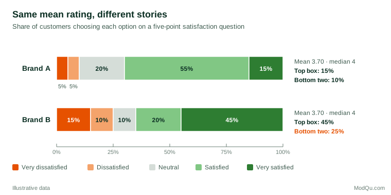
This is why many commercial measures report categories rather than means. "Top-two-box" scores report the share choosing the two most positive options, and the Net Promoter Score groups an eleven-point scale into three categories before subtracting the share of detractors from the share of promoters.
Criticisms of the typology
Data types depend on the question. Velleman and Wilkinson (1993) argued that the nominal, ordinal, interval and ratio labels are misleading when treated as fixed properties of data. The same numbers can be analysed in different ways depending on the question being asked, as Lord's jersey numbers show. Applying "permissible statistics" mechanically can hide useful structure.
Real data do not fit four boxes. Counts take only whole numbers and are often skewed, and percentages are bounded. Chrisman (1998) proposed an extended set of levels, including cyclical measures such as compass direction and time of day, and counts as a distinct type. Averaging two customers' preferred shopping hours of 23:00 and 01:00 gives 12:00, which is clearly wrong.
Measurement theory is contested. Michell (1986) identified three different philosophies of measurement behind the arguments: the representational view, in which numbers must mirror real relations between objects; the operational view, in which a measure is defined by the procedure that produces it; and the classical view, in which measurement means discovering quantities that already exist. Townsend and Ashby (1984) defended the relevance of measurement scales, arguing that ignoring them can lead to conclusions that change when the scale is changed. Hand (1996) offered a reconciliation, arguing that the relevance of the scale depends on the question: it matters most when conclusions are meant to apply to the underlying attribute rather than to the numbers as recorded.
Practical guidance for survey and business data
- Classify every variable at the design stage and record its level in the codebook.
- Collect detail where respondents can give it. Exact age, exact spend and exact counts can be grouped later. Bands cannot be ungrouped.
- Report distributions for single rating items. Show the share in each category, or top-box and bottom-box shares, alongside or instead of the mean.
- Use means for multi-item scales with care. When several items measure one idea and the summed scores have many possible values, means and standard deviations are usually reasonable.
- Check results with an ordinal method when the decision matters. If a t-test on mean ratings shows a difference, confirm it with a rank-based test or an ordinal regression.
- Avoid ratio claims without a true zero. "Twice as satisfied" or "50% more likely to agree" based on rating scores is not meaningful.
- Watch for special types. Treat time of day, direction and day of week as cyclical, and use count models for heavily skewed counts.
Common mistakes
- Averaging nominal codes. A mean region of 2.6 has no meaning.
- Treating banded data as continuous. Means of band codes for income, age or company size are distorted by unequal band widths.
- Over-applying the rules. Refusing ever to calculate a mean of ratings can discard useful information, especially for well-built multi-item scales. The aim is to avoid misleading conclusions, not to follow a rule for its own sake.
Key takeaways
Levels of measurement describe what information a set of numbers carries. Nominal data name categories, ordinal data rank them, interval data add equal spacing and ratio data add a true zero. The level guides which summaries and tests are sensible and which statements are meaningful. In survey work, classify variables early, collect detail, report distributions for single rating items and confirm important findings with ordinal methods. Used as a guide to judgement rather than a strict rulebook, Stevens's typology remains one of the most practical ideas in statistics.
References
Agresti, A. (2010). Analysis of ordinal categorical data (2nd ed.). Wiley. https://doi.org/10.1002/9780470594001
Bürkner, P.-C., & Vuorre, M. (2019). Ordinal regression models in psychology: A tutorial. Advances in Methods and Practices in Psychological Science, 2(1), 77–101. https://doi.org/10.1177/2515245918823199
Carifio, J., & Perla, R. J. (2007). Ten common misunderstandings, misconceptions, persistent myths and urban legends about Likert scales and Likert response formats and their antidotes. Journal of Social Sciences, 3(3), 106–116. https://doi.org/10.3844/jssp.2007.106.116
Chrisman, N. R. (1998). Rethinking levels of measurement for cartography. Cartography and Geographic Information Systems, 25(4), 231–242. https://doi.org/10.1559/152304098782383043
Gaito, J. (1980). Measurement scales and statistics: Resurgence of an old misconception. Psychological Bulletin, 87(3), 564–567. https://doi.org/10.1037/0033-2909.87.3.564
Hand, D. J. (1996). Statistics and the theory of measurement. Journal of the Royal Statistical Society Series A: Statistics in Society, 159(3), 445–473. https://doi.org/10.2307/2983326
Harpe, S. E. (2015). How to analyze Likert and other rating scale data. Currents in Pharmacy Teaching and Learning, 7(6), 836–850. https://doi.org/10.1016/j.cptl.2015.08.001
Jamieson, S. (2004). Likert scales: How to (ab)use them. Medical Education, 38(12), 1217–1218. https://doi.org/10.1111/j.1365-2929.2004.02012.x
Kendall, M. G. (1938). A new measure of rank correlation. Biometrika, 30(1–2), 81–93. https://doi.org/10.1093/biomet/30.1-2.81
Kruskal, W. H., & Wallis, W. A. (1952). Use of ranks in one-criterion variance analysis. Journal of the American Statistical Association, 47(260), 583–621. https://doi.org/10.1080/01621459.1952.10483441
Liddell, T. M., & Kruschke, J. K. (2018). Analyzing ordinal data with metric models: What could possibly go wrong? Journal of Experimental Social Psychology, 79, 328–348. https://doi.org/10.1016/j.jesp.2018.08.009
Lord, F. M. (1953). On the statistical treatment of football numbers. American Psychologist, 8(12), 750–751. https://doi.org/10.1037/h0063675
Mann, H. B., & Whitney, D. R. (1947). On a test of whether one of two random variables is stochastically larger than the other. The Annals of Mathematical Statistics, 18(1), 50–60. https://doi.org/10.1214/aoms/1177730491
McCullagh, P. (1980). Regression models for ordinal data. Journal of the Royal Statistical Society Series B: Statistical Methodology, 42(2), 109–127. https://doi.org/10.1111/j.2517-6161.1980.tb01109.x
Michell, J. (1986). Measurement scales and statistics: A clash of paradigms. Psychological Bulletin, 100(3), 398–407. https://doi.org/10.1037/0033-2909.100.3.398
Norman, G. (2010). Likert scales, levels of measurement and the "laws" of statistics. Advances in Health Sciences Education, 15(5), 625–632. https://doi.org/10.1007/s10459-010-9222-y
Rhemtulla, M., Brosseau-Liard, P. É., & Savalei, V. (2012). When can categorical variables be treated as continuous? A comparison of robust continuous and categorical SEM estimation methods under suboptimal conditions. Psychological Methods, 17(3), 354–373. https://doi.org/10.1037/a0029315
Stevens, S. S. (1946). On the theory of scales of measurement. Science, 103(2684), 677–680. https://doi.org/10.1126/science.103.2684.677
Sullivan, G. M., & Artino, A. R., Jr. (2013). Analyzing and interpreting data from Likert-type scales. Journal of Graduate Medical Education, 5(4), 541–542. https://doi.org/10.4300/JGME-5-4-18
Townsend, J. T., & Ashby, F. G. (1984). Measurement scales and statistics: The misconception misconceived. Psychological Bulletin, 96(2), 394–401. https://doi.org/10.1037/0033-2909.96.2.394
Velleman, P. F., & Wilkinson, L. (1993). Nominal, ordinal, interval, and ratio typologies are misleading. The American Statistician, 47(1), 65–72. https://doi.org/10.1080/00031305.1993.10475938
Wu, H., & Leung, S.-O. (2017). Can Likert scales be treated as interval scales? A simulation study. Journal of Social Service Research, 43(4), 527–532. https://doi.org/10.1080/01488376.2017.1329775