
Statistics · Foundations
Variables and Data Types in Applied Statistics
What variables are, how nominal, ordinal and numeric data differ, why the type of a variable shapes every later analysis, and how to code survey and business data so it stays useful.
Every statistical analysis starts with a decision that is easy to overlook: what kind of variable is this? A customer's region, a satisfaction rating from 1 to 5, the number of purchases last month and annual spending in dollars are all recorded as numbers or labels in a spreadsheet, yet they carry very different kinds of information. The type of a variable determines which summaries are meaningful, which charts make sense, which models apply and how results should be reported. Getting it wrong can produce averages that mean nothing, tests that lose most of their power or conclusions that reverse under a harmless change of coding.
What is a variable?
A variable is a characteristic that can take different values for different units of observation. In a customer survey, each respondent is a unit, and each question produces at least one variable: age, province, brand used most often, likelihood to recommend and so on.
Variables also play different roles. An outcome (or dependent variable) is what we want to explain or predict, such as renewal or spending, while explanatory variables (predictors, or independent variables) are those used to explain it. Some variables are derived, such as a satisfaction score built from ten items or tenure calculated from a sign-up date, and inherit the strengths and weaknesses of their inputs.
Two broad families: categorical and numeric
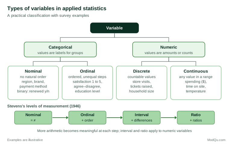
The most important division is between categorical variables, whose values are labels for groups, and numeric (or quantitative) variables, whose values are amounts or counts.
Categorical variables
A nominal variable places units into categories that have no natural order. Province, preferred brand, payment method and industry sector are nominal. A special case is the binary (or dichotomous) variable, with exactly two categories, such as whether a customer renewed.
An ordinal variable has categories with a meaningful order but no fixed distance between them. Education level, a "poor / fair / good / excellent" rating and agreement on a five-point scale from "strongly disagree" to "strongly agree" are ordinal. We know that "good" is better than "fair", but not whether the step from "fair" to "good" is the same size as the step from "good" to "excellent".
Numeric variables
A discrete numeric variable takes separate, countable values, usually whole numbers: the number of store visits, children in a household or support tickets raised. A continuous variable can, in principle, take any value within a range: weight, time on a website, temperature or spending. In practice the line is partly a matter of convenience: spending recorded to the cent behaves as continuous for almost every purpose.
Numeric variables can be further split by the nature of their zero point, which leads to the best-known classification in the field.
Stevens's levels of measurement
The psychologist S. S. Stevens proposed that measurements fall into four scales: nominal, ordinal, interval and ratio (Stevens, 1946). He defined each scale by the transformations that leave its information unchanged, and argued that each scale permits a particular set of statistics. On an interval scale, differences are meaningful but zero is arbitrary, as with temperature in degrees Celsius: 20 °C is not "twice as warm" as 10 °C. On a ratio scale, zero means "none of the quantity", so ratios are meaningful: a customer who spends $200 has spent twice as much as one who spends $100.
| Level | What is meaningful | Transformations that preserve it | Typical summaries | Survey and business examples |
|---|---|---|---|---|
| Nominal | Equality of categories | Any one-to-one relabelling | Counts, percentages, mode | Region, brand, channel |
| Ordinal | Order | Any order-preserving change | Median, percentiles | Rating scales, education level |
| Interval | Differences | Linear: a + bx | Mean, standard deviation | Temperature in °C, calendar year |
| Ratio | Differences and ratios | Multiplication: bx | Geometric mean, coefficient of variation, plus all of the above | Spending, units sold, time on site |
Each level includes the information of the levels above it in the table, so a ratio variable can always be summarised with a median or grouped into categories, but not the other way round.
A guide, not a rulebook
Stevens's scheme is a useful first check. Its stronger claim, that the scale of a variable dictates which statistics are "permissible", has been disputed almost from the start.
Lord (1953) made the point with a satire about football jersey numbers. In the story, first-year students complain that the numbered jerseys they have been sold carry unusually low numbers. A statistician averages the numbers and tests whether they are lower than chance would suggest, setting aside the objection that jersey numbers are only nominal labels, on the grounds that the numbers themselves cannot know where they came from. For the question being asked, the mean was a perfectly sensible tool. The lesson is that the question matters as much as the label attached to the variable.
Velleman and Wilkinson (1993) went further, arguing that the nominal, ordinal, interval and ratio typology is misleading when used as a rule for choosing methods. Many real variables do not fit neatly into one level, the same data can be treated at different levels for different purposes, and rigid rules can steer analysts away from good analyses. Michell (1986) traced the disagreement to different theories of what measurement is, and Kampen and Swyngedouw (2000) reviewed the long-running "ordinal controversy" over when ordinal data may be analysed with interval methods.
The sensible position for applied work is that measurement level is a strong guide to what a statistic means, not a law about what may be calculated. A mean of region codes is meaningless because changing the arbitrary codes would change the answer. A mean of five-point ratings can be informative, but it rests on an assumption about equal spacing that should be stated and, where it matters, checked.
The Likert debate
Nowhere is the disagreement sharper than with rating scales, the workhorse of survey research. Jamieson (2004) argued that responses to Likert items are ordinal, that the intervals between categories cannot be assumed equal, and that means and standard deviations are therefore inappropriate. Norman (2010) replied that parametric methods such as t tests and regression are robust to violations of their assumptions, and that analysing Likert data with them rarely leads to wrong conclusions.
Part of the confusion comes from mixing up a single Likert item with a Likert scale, which is the sum or average of several items measuring the same idea. Carifio and Perla (2007) stressed this distinction and argued that multi-item scales can reasonably be treated as interval data. Sullivan and Artino (2013) and Harpe (2015) offer similar practical guidance: report single items with frequencies and medians, and treat well-constructed multi-item scales as approximately continuous.
There are real risks in treating ordinal responses as if they were metric, however. Liddell and Kruschke (2018) showed through analysis and examples that doing so can produce false positives, missed effects and even reversals in the direction of an effect, particularly when groups differ in variability or when responses pile up at one end of the scale. Models built for ordered outcomes avoid this. The proportional odds model (McCullagh, 1980) treats an ordinal response as a set of ordered thresholds on an underlying continuum, and Bürkner and Vuorre (2019) give an accessible tutorial on this and related ordinal regression models.
For business reporting, a practical compromise is to show the full distribution alongside any mean, and to confirm key conclusions with an ordinal method.
Data types in software
Statistical type and storage type are not the same thing. Software stores values as integers, decimals, text strings, dates, logical (true/false) values and, in many packages, as factors or labelled categories. A province coded 1 to 13 is stored as an integer, but it is still nominal. A five-point rating stored as text ("Agree", "Strongly agree") is still ordinal, but the software will sort it alphabetically unless the order is declared. A postal code looks numeric but must be stored as text, or leading zeros and letters will be lost.
Common errors at this stage include special codes such as 99 for "don't know" treated as genuine numbers, dates imported as text or converted into serial numbers, and identifiers summed or averaged. Wickham (2014) set out the principles of tidy data: each variable forms a column, each observation forms a row and each type of observational unit forms a table. Broman and Woo (2018) give practical rules for spreadsheets that support the same goal: be consistent in codes and names, write dates in the ISO format YYYY-MM-DD, put one piece of information in each cell, never use colour or highlighting to store information, and keep a data dictionary that describes every variable.
A worked example: coding a customer survey
Suppose a hypothetical retailer runs a short survey of 800 customers. Before analysis, the team writes a data dictionary that records the statistical type of each variable and how it will be summarised.
| Variable | Question or source | Statistical type | Stored as | Summary to report |
|---|---|---|---|---|
| resp_id | System identifier | Identifier (not analysed) | Text | None |
| region | Region of residence | Nominal | Labelled category | Counts and percentages |
| member | Loyalty programme member? | Binary | Logical | Percentage "yes" |
| sat_overall | Overall satisfaction, 1 to 5 | Ordinal | Ordered category | Distribution, median, top-two-box % |
| sat_index | Mean of six satisfaction items | Approximately continuous | Decimal | Mean, standard deviation |
| visits_3m | Store visits in last 3 months | Discrete count | Integer | Mean, median, distribution |
| spend_12m | Spending in last 12 months ($) | Continuous ratio | Decimal | Median, mean, percentiles |
| nps_raw | Likelihood to recommend, 0 to 10 | Ordinal (often treated as numeric) | Integer | Distribution and NPS bands |
Several choices in this illustrative dictionary deserve comment. The identifier is kept as text so that no one accidentally analyses it. Overall satisfaction is held as an ordered category, so software sorts it correctly and will not average it by default. Spending is reported with the median as well as the mean, because spending data are usually strongly right-skewed: a few large customers can pull the mean well above what a typical customer spends. "Don't know" and "prefer not to say" answers are stored as missing values with a separate code that records the reason, rather than as numbers that might enter a calculation.
The cost of throwing information away
A common habit in business reporting is to turn numeric variables into categories: splitting customers into "high" and "low" spenders at the median, or turning age into a yes/no "under 35" flag. This discards more information than most people expect.
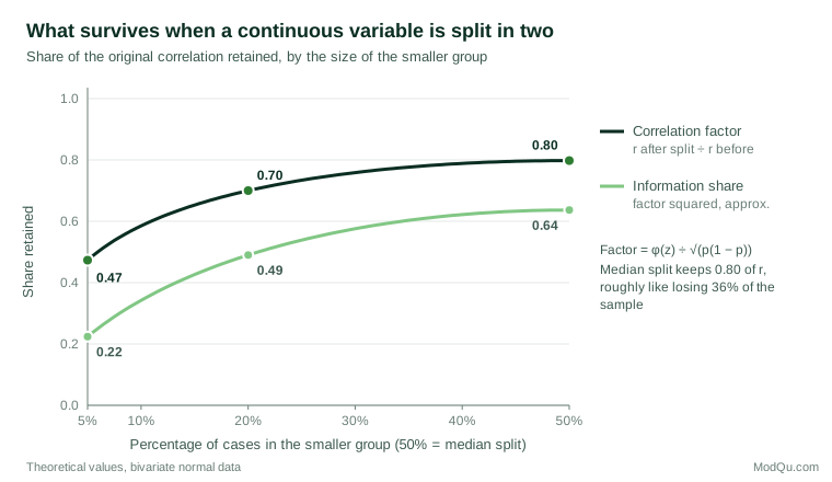
Cohen (1983) showed that splitting a normally distributed variable at its median reduces its correlation with another variable to about 0.8 of its original value. More generally, if X and Y follow a bivariate normal distribution with correlation r, and X is split so that a proportion p of units fall in one group, the correlation with the new binary variable is:
rsplit = r × φ(zp) ÷ √(p(1 − p))
where φ is the standard normal density and zp is the cut-off point. For a median split (p = 0.5) the factor is 0.798. Uneven splits are worse: when only 10% of units fall in the smaller group, the factor drops to 0.585. Because the statistical information in a correlation is roughly proportional to its square, a median split behaves much like throwing away more than a third of the sample.
MacCallum et al. (2002) reviewed the practice in psychology and found that the arguments usually given for dichotomisation rarely hold, while the costs include lost power, underestimated effect sizes and, in some situations with two predictors, spurious significant effects. In regression modelling, Royston et al. (2006) described dichotomising continuous predictors as "a bad idea", noting that it hides non-linear relationships, creates artificial jumps at the cut-off and leaves residual confounding when the variable is used as a control. Altman and Royston (2006) summarised the same costs for a general audience; the practical advice is to analyse the variable in its original form and create bands only for presentation.
Other decisions that change a variable's type
Missing and non-substantive answers
A missing value is not a value of zero and not a category like any other. Rubin (1976) set out the framework that is still used to think about missingness: whether the chance that a value is missing depends on nothing in the data, only on observed values, or on the missing value itself. This determines whether dropping incomplete cases is safe. Little and Rubin (2019) give a full treatment of methods such as multiple imputation. In surveys, "don't know" can be informative in its own right, for example as a measure of awareness, so it is often best kept as a separate category for descriptive reporting and treated as missing for modelling.
Transformations and rescaling
Skewed ratio variables such as spending or income are often analysed on a logarithmic scale, which turns multiplicative differences into additive ones. Box and Cox (1964) proposed a family of power transformations that includes the logarithm as a special case. Transformation changes how results should be read: an effect on log spending is an effect in percentage terms. When numeric and binary predictors appear in the same model, Gelman (2008) suggested dividing numeric inputs by two standard deviations so that their coefficients are roughly comparable with those of binary inputs.
The number of response categories
The type of a survey variable is decided at the questionnaire design stage, long before analysis. An open numeric question ("How many times did you visit?") yields a count, while banded options ("none, 1 to 2, 3 to 5, 6 or more") yield an ordinal variable that cannot be turned back into counts. Krosnick (1999) reviewed evidence on question design, including how the format of response options affects data quality. For agree–disagree scales, Revilla et al. (2014) found that five answer categories gave higher measurement quality than seven or eleven.
Practical guidance for survey and business data
- Classify every variable before analysis. Record its statistical type, storage type, valid values and missing-value codes in a data dictionary.
- Separate codes from quantities. Numbers used as labels, such as region codes, store numbers and identifiers, should be stored so that they cannot be averaged by accident.
- Keep numeric data numeric. Collect counts and amounts as numbers where respondents can answer accurately, and create bands only for presentation.
- Report distributions for rating items. Show the percentage in each category, or top-box and bottom-box shares, alongside any mean.
- Use methods that fit the outcome. Logistic regression for binary outcomes, ordinal models for ordered ratings, count models for counts and transformations for skewed amounts.
- Check robustness when it matters. If a decision rests on a difference in mean ratings, confirm it with an ordinal method or a comparison of distributions.
Common mistakes
- Treating special codes as data. A "99 = don't know" code included in a mean can distort it badly.
- Dichotomising without need. Median splits and arbitrary cut-offs throw away information and can create artificial effects.
- Over-reading small differences in mean ratings. A shift from 3.9 to 4.0 on a five-point scale may reflect a change at one end of the distribution only, and may not hold under an ordinal analysis.
- Mixing up storage and meaning. That a variable is stored as a number does not make it numeric in the statistical sense.
Key takeaways
The type of a variable is the first fact an analyst needs to know, and it shapes every later step, from the choice of summary to the choice of model. Stevens's levels of measurement are a valuable guide to what a statistic means, but not a strict rulebook, and the debate over rating scales shows that informed judgement matters more than labels. Clear coding, a written data dictionary, keeping numeric variables numeric and choosing methods that fit each outcome prevent most errors that start with a misclassified variable.
References
Altman, D. G., & Royston, P. (2006). The cost of dichotomising continuous variables. BMJ, 332(7549), 1080. https://doi.org/10.1136/bmj.332.7549.1080
Box, G. E. P., & Cox, D. R. (1964). An analysis of transformations. Journal of the Royal Statistical Society Series B: Statistical Methodology, 26(2), 211–243. https://doi.org/10.1111/j.2517-6161.1964.tb00553.x
Broman, K. W., & Woo, K. H. (2018). Data organization in spreadsheets. The American Statistician, 72(1), 2–10. https://doi.org/10.1080/00031305.2017.1375989
Bürkner, P.-C., & Vuorre, M. (2019). Ordinal regression models in psychology: A tutorial. Advances in Methods and Practices in Psychological Science, 2(1), 77–101. https://doi.org/10.1177/2515245918823199
Carifio, J., & Perla, R. J. (2007). Ten common misunderstandings, misconceptions, persistent myths and urban legends about Likert scales and Likert response formats and their antidotes. Journal of Social Sciences, 3(3), 106–116. https://doi.org/10.3844/jssp.2007.106.116
Cohen, J. (1983). The cost of dichotomization. Applied Psychological Measurement, 7(3), 249–253. https://doi.org/10.1177/014662168300700301
Gelman, A. (2008). Scaling regression inputs by dividing by two standard deviations. Statistics in Medicine, 27(15), 2865–2873. https://doi.org/10.1002/sim.3107
Harpe, S. E. (2015). How to analyze Likert and other rating scale data. Currents in Pharmacy Teaching and Learning, 7(6), 836–850. https://doi.org/10.1016/j.cptl.2015.08.001
Jamieson, S. (2004). Likert scales: How to (ab)use them. Medical Education, 38(12), 1217–1218. https://doi.org/10.1111/j.1365-2929.2004.02012.x
Kampen, J., & Swyngedouw, M. (2000). The ordinal controversy revisited. Quality and Quantity, 34(1), 87–102. https://doi.org/10.1023/A:1004785723554
Krosnick, J. A. (1999). Survey research. Annual Review of Psychology, 50(1), 537–567. https://doi.org/10.1146/annurev.psych.50.1.537
Liddell, T. M., & Kruschke, J. K. (2018). Analyzing ordinal data with metric models: What could possibly go wrong? Journal of Experimental Social Psychology, 79, 328–348. https://doi.org/10.1016/j.jesp.2018.08.009
Little, R. J. A., & Rubin, D. B. (2019). Statistical analysis with missing data (3rd ed.). Wiley. https://doi.org/10.1002/9781119482260
Lord, F. M. (1953). On the statistical treatment of football numbers. American Psychologist, 8(12), 750–751. https://doi.org/10.1037/h0063675
MacCallum, R. C., Zhang, S., Preacher, K. J., & Rucker, D. D. (2002). On the practice of dichotomization of quantitative variables. Psychological Methods, 7(1), 19–40. https://doi.org/10.1037/1082-989X.7.1.19
McCullagh, P. (1980). Regression models for ordinal data. Journal of the Royal Statistical Society Series B: Statistical Methodology, 42(2), 109–127. https://doi.org/10.1111/j.2517-6161.1980.tb01109.x
Michell, J. (1986). Measurement scales and statistics: A clash of paradigms. Psychological Bulletin, 100(3), 398–407. https://doi.org/10.1037/0033-2909.100.3.398
Norman, G. (2010). Likert scales, levels of measurement and the "laws" of statistics. Advances in Health Sciences Education, 15(5), 625–632. https://doi.org/10.1007/s10459-010-9222-y
Revilla, M. A., Saris, W. E., & Krosnick, J. A. (2014). Choosing the number of categories in agree–disagree scales. Sociological Methods & Research, 43(1), 73–97. https://doi.org/10.1177/0049124113509605
Royston, P., Altman, D. G., & Sauerbrei, W. (2006). Dichotomizing continuous predictors in multiple regression: A bad idea. Statistics in Medicine, 25(1), 127–141. https://doi.org/10.1002/sim.2331
Rubin, D. B. (1976). Inference and missing data. Biometrika, 63(3), 581–592. https://doi.org/10.1093/biomet/63.3.581
Stevens, S. S. (1946). On the theory of scales of measurement. Science, 103(2684), 677–680. https://doi.org/10.1126/science.103.2684.677
Sullivan, G. M., & Artino, A. R. (2013). Analyzing and interpreting data from Likert-type scales. Journal of Graduate Medical Education, 5(4), 541–542. https://doi.org/10.4300/JGME-5-4-18
Velleman, P. F., & Wilkinson, L. (1993). Nominal, ordinal, interval, and ratio typologies are misleading. The American Statistician, 47(1), 65–72. https://doi.org/10.1080/00031305.1993.10475938
Wickham, H. (2014). Tidy data. Journal of Statistical Software, 59(10). https://doi.org/10.18637/jss.v059.i10