
Statistics · Foundations
Probability Theory for Non-Mathematicians
A plain-language guide to the ideas of probability that matter in business and survey work: the basic rules, conditional probability, Bayes' theorem, expected value, sample size and the intuitive traps that mislead decisions.
Every forecast, margin of error, risk score and test result rests on probability. A survey report that says 42% of customers intend to switch "plus or minus three points" is a probability statement. So is a churn model that rates a customer as "high risk", a sales pipeline that weights deals by their chance of closing, and a weather app that shows a 70% chance of rain. Yet many managers who use these results every day were never shown the handful of ideas that make them work. This article sets out those ideas without assuming any mathematical background, using examples from survey research and everyday business data.
What a probability is
A probability is a number between 0 and 1 (or 0% and 100%) that expresses how likely something is. A probability of 0 means the event cannot happen, 1 means it is certain, and 0.5 means it is as likely to happen as not. What the number means has been debated for more than three centuries, and different interpretations suit different problems (Hacking, 2001, 2006).
Three interpretations are worth knowing:
- Classical probability counts equally likely outcomes. A fair die has six faces, so the chance of rolling a four is 1 in 6. This suits games of chance and randomised procedures such as drawing a simple random sample.
- Frequency probability defines a probability as the long-run proportion of times an event occurs when a process is repeated. If 3% of online orders over many months are returned, the probability that a new order is returned is about 3%. Most survey statistics rest on this view.
- Subjective or Bayesian probability treats a probability as a degree of belief, given the evidence available. A sales director who says there is a 60% chance of winning a contract is not describing a long run of identical contracts; she is expressing a judgement that can be updated.
All three follow the same rules. The practical point is to know, when a probability is quoted, whether it comes from counting, from data or from judgement, because each can go wrong in different ways.
The basic rules
Modern probability theory rests on a few axioms set out by Andrey Kolmogorov in the 1930s, which introductory texts present in accessible form (Blitzstein & Hwang, 2019). For practical purposes, four rules cover most needs.
1. The complement rule. The probability that an event does not happen is one minus the probability that it does:
P(not A) = 1 − P(A)
If 18% of customers churned last year, 82% stayed. The chance of at least one complaint in a batch is usually easiest to find as one minus the chance of no complaints.
2. The addition rule. The probability that at least one of two events happens is the sum of their probabilities, minus the probability that both happen (which would otherwise be counted twice):
P(A or B) = P(A) + P(B) − P(A and B)
Suppose, in a hypothetical survey, 40% of respondents use Brand A, 30% use Brand B and 18% use both. The share using at least one of the two brands is 40% + 30% − 18% = 52%, not 70%.
3. Conditional probability. The probability of A given that B has happened, written P(A | B), restricts attention to the cases where B is true:
P(A | B) = P(A and B) ÷ P(B)
In the same survey, the probability that a Brand A user also uses Brand B is 18% ÷ 40% = 45%. Among all respondents only 30% use Brand B, so knowing that someone uses Brand A changes the probability that they use Brand B. Conditional probability is the formal language of "among those who…", and of almost every cross-tabulation.
4. The multiplication rule and independence. The probability that both A and B happen is the probability of A times the probability of B given A:
P(A and B) = P(A) × P(B | A)
Two events are independent when knowing one tells you nothing about the other, so that P(B | A) = P(B). Only then does the familiar shortcut P(A and B) = P(A) × P(B) apply. In the brand example, if the two brands were used independently, we would expect 40% × 30% = 12% to use both. The observed 18% shows that the two behaviours are linked, perhaps because both appeal to heavy category buyers.
Assuming independence that does not exist is a common error. Two back-up systems, each with a 1% chance of failure, both fail with probability 1 in 10,000 only if their failures are unrelated; if they share a power supply, the risk is far higher.
Conditional probability in survey data
Conditional probabilities are everywhere in survey and customer data, and they are easy to confuse. The probability that a customer is dissatisfied given that they complained is not the same as the probability that a customer complained given that they are dissatisfied. The first might be 90%; the second might be 5%, because most dissatisfied customers never complain, they simply leave.
Confusing P(A | B) with P(B | A) is sometimes called the fallacy of the transposed conditional. A common statistical version concerns the p-value. A p-value is the probability of seeing data at least as extreme as those observed if there is no real effect. It is not the probability that there is no real effect given the data. The American Statistical Association's statement on p-values makes this point directly: a p-value does not measure the probability that the studied hypothesis is true (Wasserstein & Lazar, 2016).
A useful habit when reading any percentage is to ask, "percentage of what?"
Bayes' theorem and the base-rate trap
Bayes' theorem, first published after the death of the Reverend Thomas Bayes (Bayes, 1763), shows how to reverse a conditional probability. It combines what was known before seeing the evidence (the prior probability, or base rate) with how strongly the evidence points one way or the other:
P(A | B) = P(B | A) × P(A) ÷ P(B)
The idea is intuitive once it is set out with counts. Consider a hypothetical churn-warning model used by a subscription business:
- 5% of customers will cancel in the next quarter (the base rate).
- The model flags 80% of customers who will cancel (its sensitivity).
- It also wrongly flags 10% of customers who will stay (its false-positive rate).
If a customer is flagged, what is the probability that they will actually cancel? Many people answer 80%. The correct answer is about 30%.
To see why, imagine 10,000 customers. Of these, 500 will cancel and 9,500 will stay. The model flags 80% of the 500, which is 400 true warnings. It also flags 10% of the 9,500 who stay, which is 950 false alarms. In total 1,350 customers are flagged, and only 400 of them will cancel: 400 ÷ 1,350 ≈ 30%.
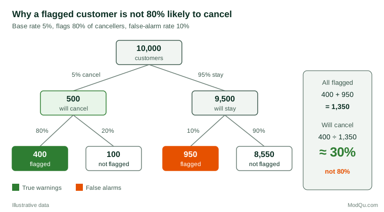
This is the base-rate trap: when an event is rare, even a fairly accurate test produces many more false positives than true positives. The classic demonstration involved physicians and medical students at a Harvard teaching hospital, who were asked about a test for a disease with a prevalence of 1 in 1,000 and a 5% false-positive rate. The correct answer was about 2%, yet fewer than one in five gave it, and the most common answer was 95% (Casscells et al., 1978).
The remedy is not more mathematics but a better format. Gigerenzer and Hoffrage (1995) showed that people reason far more accurately when the same information is given as natural frequencies ("400 out of 1,350") rather than as conditional probabilities ("80% sensitivity, 10% false-positive rate"). Later work found the same improvement among doctors and legal professionals (Hoffrage et al., 2000), and a major review recommends natural frequencies and absolute risks as standard practice in communicating health statistics (Gigerenzer et al., 2007). The same advice applies to fraud alerts, lead scores and quality inspections.
The same logic applies to research. If few of the hypotheses tested are true, many "significant" findings will be false positives; Ioannidis (2005) used this reasoning to argue that most published findings in some fields are likely to be false. For a business running many A/B tests, a significant result on an unlikely idea deserves replication.
Random variables and expected value
A random variable is a quantity whose value depends on chance: the number of customers who respond to a mailing, the revenue from a deal, the score a respondent gives on a ten-point scale. Its probability distribution lists the possible values and how likely each one is. Its expected value is the probability-weighted average of those values, the average result over many repetitions:
E(X) = Σ x × P(X = x)
Expected value is the basic tool for decisions under uncertainty. Suppose, hypothetically, that a direct-marketing offer costs $1.50 per contact, 2% of contacts respond, and each response brings a profit margin of $60. The expected margin per contact is 0.02 × $60 = $1.20, which is less than the $1.50 cost. On average the campaign loses about 30 cents per contact, even though each individual response is very profitable. If targeting could raise the response rate to 3%, the expected margin would rise to $1.80 and the campaign would pay.
Two cautions apply. First, the expected value is an average, not a forecast of any single outcome. A pipeline with ten deals each at a 10% chance of closing has an expected value of one closed deal, but there is roughly a one-in-three chance that none close at all (0.9 multiplied by itself ten times is about 0.35). Second, expected value ignores the spread of outcomes. Two projects with the same expected profit can carry very different risks, and decision-makers are usually right to care about the downside as well as the average.
The law of large numbers and the trouble with small samples
The law of large numbers states that, as the number of independent observations grows, the observed proportion of an event gets closer and closer to its true probability. Toss a fair coin ten times and you may well see seven heads; toss it ten thousand times and the share of heads will almost certainly be very close to 50%.
The law says nothing about short runs, however, and small samples vary far more than intuition suggests. Tversky and Kahneman (1971) found that even trained research psychologists placed too much faith in results from small samples, expecting them to resemble the population as closely as large ones do.
Figure 2 shows the effect. It follows a hypothetical survey in which the true share of customers who would recommend a product is 30%. With 20 or 30 responses the running estimate wanders well away from 30%; by 1,000 responses it stays close.
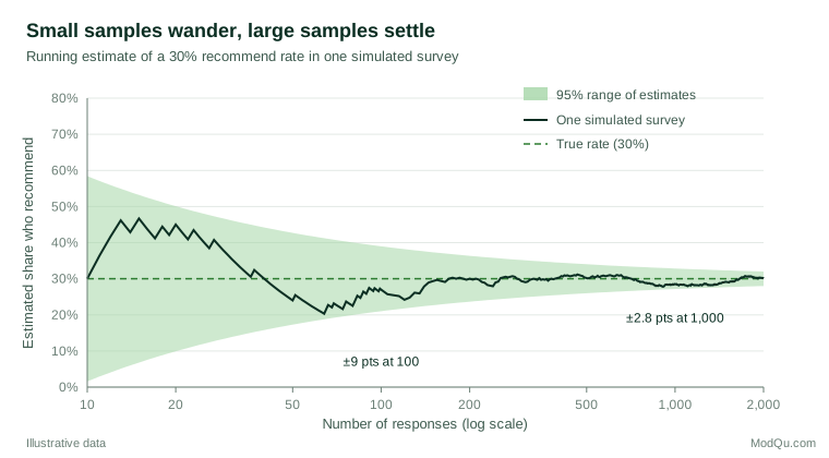
The width of the band follows a simple pattern. For a proportion p estimated from a simple random sample of n people, the standard error is:
SE = √( p × (1 − p) ÷ n )
and the familiar 95% margin of error is about 1.96 times the standard error. With p = 30%, the margin is about ±9 percentage points at 100 responses, ±4.5 points at 400 and ±2.8 points at 1,000. Quadrupling the sample only halves the margin of error, which is why precision becomes expensive. For small samples or proportions near 0% or 100%, the simple formula performs poorly, and better intervals such as the Wilson score interval should be used (Wilson, 1927; Agresti & Coull, 1998).
Two further points matter in survey work. First, these formulas assume probability sampling, in which every member of the population has a known, non-zero chance of selection; complex designs with clusters, strata or weights need their own variance calculations (Lohr, 2021). Second, the margin of error covers only random sampling variation. It says nothing about bias from poor coverage, non-response or leading questions, which no increase in sample size can fix.
Where intuition goes wrong
Human judgement about chance is not random; it errs in predictable directions. Tversky and Kahneman (1974) described several mental shortcuts, or heuristics, that usually serve people well but lead to systematic mistakes with probabilities.
Judging by resemblance
People often judge the probability of an event by how much it resembles a typical case, rather than by how often such cases occur. Kahneman and Tversky (1972) called this the representativeness heuristic. Birth orders in a family that look random, such as girl-boy-girl-boy-boy-girl, are judged more likely than equally probable orders that look patterned.
The conjunction fallacy
A combination of two events can never be more probable than either event alone, because every case in which both happen is also a case in which the first happens. Yet in a famous experiment, most participants judged that "Linda is a bank teller and is active in the feminist movement" was more probable than "Linda is a bank teller", after reading a description that fitted the feminist stereotype (Tversky & Kahneman, 1983). Each extra detail makes a story more plausible but less likely. In strategy terms, if five independent assumptions each have an 80% chance of holding, the chance that all five hold is only about 33%.
Streaks and the gambler's fallacy
The gambler's fallacy is the belief that after a run of one outcome, the opposite outcome is "due". The opposite belief, that a run of success makes further success more likely, has a more complicated story. Gilovich et al. (1985) found no evidence that basketball players had "hot hands" beyond what chance would produce. Three decades later, Miller and Sanjurjo (2018) showed that the standard way of measuring streaks in short sequences contains a subtle bias, and that correcting it reveals evidence of a modest hot-hand effect after all. Probability can trip up experts too.
Coincidences
Surprising coincidences are much more common than they seem, because there are so many opportunities for them. In a group of only 23 people, the chance that at least two share a birthday is just over 50%. Diaconis and Mosteller (1989) described this as part of a "law of truly large numbers": with a large enough number of opportunities, almost any outrageous event is likely to happen somewhere. A business monitoring hundreds of metrics across dozens of regions will see several apparently remarkable spikes every month by chance alone.
Overconfidence
People also tend to be more certain than the evidence justifies. In studies of general-knowledge questions, Fischhoff et al. (1977) found that people who described themselves as certain of an answer were still wrong a substantial share of the time. Overconfident forecasts produce ranges that are far too narrow.
Probability in forecasting and business decisions
Probabilities are only useful if they are reliable. A forecaster is well calibrated if, among all the occasions on which she says "70%", the event happens about 70% of the time. Weather forecasting offers the best-known success story: probability-of-precipitation forecasts in the United States have long been found to be well calibrated (Murphy & Winkler, 1984).
The same discipline can be applied to sales forecasts, project estimates and market predictions. The Brier score, proposed for weather forecasts, measures accuracy as the average squared difference between the forecast probability and the outcome, coded 1 if the event happened and 0 if it did not (Brier, 1950):
Brier score = (1 ÷ N) × Σ (fi − oi)²
Lower scores are better. A forecaster who always says 50% scores 0.25; a perfect forecaster scores 0. Recording and scoring probability forecasts is a cheap way to learn whether judgements can be trusted.
Communicating probability matters as much as calculating it. Verbal phrases such as "likely" mean different things to different readers. Spiegelhalter et al. (2011) review ways of presenting uncertainty visually, from fan charts to icon arrays, and Spiegelhalter (2017) recommends expected frequencies ("about 3 in 100 customers"), clear statements of the reference group, and absolute rather than only relative changes. "Halving the defect rate" is less impressive if it falls from 2 to 1 in 10,000.
Practical guidance for survey and business data
- State the reference group. Every probability or percentage is conditional on something. Say who is included, over what period and under what assumptions.
- Check the direction of the conditional. Before acting on a statement like "80% of churners were flagged", ask for the reverse: what share of flagged customers actually churned?
- Start with the base rate. For any prediction, screening tool or test, find out how common the event is in the first place. Rare events produce many false positives.
- Use natural frequencies. Translate probabilities into counts out of a round number, such as 1,000 customers, when presenting to colleagues or clients.
- Do not assume independence. Ask whether events share a common cause before multiplying their probabilities together.
- Respect sample size. Treat results from small subgroups with caution, report margins of error, and use appropriate intervals for small samples or extreme proportions.
- Remember what the margin of error leaves out. It reflects sampling variation only, not coverage, non-response or measurement problems.
- Expect coincidences. When many comparisons are made, some will look remarkable by chance. Confirm surprising findings with fresh data before acting.
- Score your forecasts. Record probability forecasts and compare them with outcomes so that calibration can improve over time.
Key takeaways
Probability theory need not be intimidating. A probability is a number between 0 and 1 that can describe equally likely outcomes, long-run frequencies or reasoned judgements, and in each case it follows the same few rules. Conditional probability is the language of "among those who", and reversing a conditional requires Bayes' theorem and attention to the base rate. Expected value supports decisions but hides risk. Large samples settle down; small samples wander. And human intuition, however experienced, makes predictable mistakes with chance, which is why counting, scoring and plain natural frequencies are such valuable habits. For anyone who commissions, reads or presents survey research and business data, these ideas are the foundation on which every other statistical method is built.
References
Agresti, A., & Coull, B. A. (1998). Approximate is better than "exact" for interval estimation of binomial proportions. The American Statistician, 52(2), 119–126. https://doi.org/10.1080/00031305.1998.10480550
Bayes, T. (1763). An essay towards solving a problem in the doctrine of chances. Philosophical Transactions of the Royal Society of London, 53, 370–418. https://doi.org/10.1098/rstl.1763.0053
Blitzstein, J. K., & Hwang, J. (2019). Introduction to probability (2nd ed.). Chapman and Hall/CRC. https://doi.org/10.1201/9780429428357
Brier, G. W. (1950). Verification of forecasts expressed in terms of probability. Monthly Weather Review, 78(1), 1–3. https://doi.org/10.1175/1520-0493(1950)078<0001:VOFEIT>2.0.CO;2
Casscells, W., Schoenberger, A., & Graboys, T. B. (1978). Interpretation by physicians of clinical laboratory results. New England Journal of Medicine, 299(18), 999–1001. https://doi.org/10.1056/NEJM197811022991808
Diaconis, P., & Mosteller, F. (1989). Methods for studying coincidences. Journal of the American Statistical Association, 84(408), 853–861. https://doi.org/10.1080/01621459.1989.10478847
Fischhoff, B., Slovic, P., & Lichtenstein, S. (1977). Knowing with certainty: The appropriateness of extreme confidence. Journal of Experimental Psychology: Human Perception and Performance, 3(4), 552–564. https://doi.org/10.1037/0096-1523.3.4.552
Gigerenzer, G., Gaissmaier, W., Kurz-Milcke, E., Schwartz, L. M., & Woloshin, S. (2007). Helping doctors and patients make sense of health statistics. Psychological Science in the Public Interest, 8(2), 53–96. https://doi.org/10.1111/j.1539-6053.2008.00033.x
Gigerenzer, G., & Hoffrage, U. (1995). How to improve Bayesian reasoning without instruction: Frequency formats. Psychological Review, 102(4), 684–704. https://doi.org/10.1037/0033-295X.102.4.684
Gilovich, T., Vallone, R., & Tversky, A. (1985). The hot hand in basketball: On the misperception of random sequences. Cognitive Psychology, 17(3), 295–314. https://doi.org/10.1016/0010-0285(85)90010-6
Hacking, I. (2001). An introduction to probability and inductive logic. Cambridge University Press. https://doi.org/10.1017/CBO9780511801297
Hacking, I. (2006). The emergence of probability: A philosophical study of early ideas about probability, induction and statistical inference (2nd ed.). Cambridge University Press. https://doi.org/10.1017/CBO9780511817557
Hoffrage, U., Lindsey, S., Hertwig, R., & Gigerenzer, G. (2000). Communicating statistical information. Science, 290(5500), 2261–2262. https://doi.org/10.1126/science.290.5500.2261
Ioannidis, J. P. A. (2005). Why most published research findings are false. PLoS Medicine, 2(8), Article e124. https://doi.org/10.1371/journal.pmed.0020124
Kahneman, D., & Tversky, A. (1972). Subjective probability: A judgment of representativeness. Cognitive Psychology, 3(3), 430–454. https://doi.org/10.1016/0010-0285(72)90016-3
Lohr, S. L. (2021). Sampling: Design and analysis (3rd ed.). Chapman and Hall/CRC. https://doi.org/10.1201/9780429298899
Miller, J. B., & Sanjurjo, A. (2018). Surprised by the hot hand fallacy? A truth in the law of small numbers. Econometrica, 86(6), 2019–2047. https://doi.org/10.3982/ECTA14943
Murphy, A. H., & Winkler, R. L. (1984). Probability forecasting in meteorology. Journal of the American Statistical Association, 79(387), 489–500. https://doi.org/10.1080/01621459.1984.10478075
Spiegelhalter, D. (2017). Risk and uncertainty communication. Annual Review of Statistics and Its Application, 4(1), 31–60. https://doi.org/10.1146/annurev-statistics-010814-020148
Spiegelhalter, D., Pearson, M., & Short, I. (2011). Visualizing uncertainty about the future. Science, 333(6048), 1393–1400. https://doi.org/10.1126/science.1191181
Tversky, A., & Kahneman, D. (1971). Belief in the law of small numbers. Psychological Bulletin, 76(2), 105–110. https://doi.org/10.1037/h0031322
Tversky, A., & Kahneman, D. (1974). Judgment under uncertainty: Heuristics and biases. Science, 185(4157), 1124–1131. https://doi.org/10.1126/science.185.4157.1124
Tversky, A., & Kahneman, D. (1983). Extensional versus intuitive reasoning: The conjunction fallacy in probability judgment. Psychological Review, 90(4), 293–315. https://doi.org/10.1037/0033-295X.90.4.293
Wasserstein, R. L., & Lazar, N. A. (2016). The ASA statement on p-values: Context, process, and purpose. The American Statistician, 70(2), 129–133. https://doi.org/10.1080/00031305.2016.1154108
Wilson, E. B. (1927). Probable inference, the law of succession, and statistical inference. Journal of the American Statistical Association, 22(158), 209–212. https://doi.org/10.1080/01621459.1927.10502953