
Statistics · Foundations
The Law of Large Numbers and Its Practical Meaning
Why averages from larger random samples settle near the true value, how fast that happens, and why a large sample cannot rescue data that were collected with bias.
Every survey estimate rests on a simple promise: if you ask enough people, chosen at random, the average of their answers will be close to the average for everyone. That promise has a name, the law of large numbers, and it is one of the oldest results in probability. Jacob Bernoulli spent some twenty years on a proof, which was published after his death in 1713 (Bernoulli, 2006). It explains why sampling works, and it is widely misread.
What the law says
Suppose we draw observations independently from a population with a true mean μ, such as the share of customers who would buy a new product. The sample mean x̄n after n observations is a random quantity: a different sample would give a different value. The weak law of large numbers states that, as n grows, the probability that x̄n differs from μ by more than any fixed amount shrinks towards zero. The strong law makes the stronger claim that the sequence of sample means will, with probability one, eventually settle at μ (Wasserman, 2004).
For practical work, the important part is not the limit but the speed. If each observation has standard deviation σ, the standard error of the mean is:
SE(x̄n) = σ ÷ √n
For a proportion p, σ = √(p(1 − p)). The standard error falls with the square root of the sample size, so halving the error requires four times as many respondents. This square-root rule is the quantitative heart of the law, and Wainer (2007) calls it "the most dangerous equation" because ignoring it has led to so many costly mistakes.
A worked example
Imagine a hypothetical product whose true purchase rate among target customers is 30%. Figure 1 follows three simulated samples as respondents are added one at a time. With a handful of respondents, the running rate jumps around wildly: after two people it can be 0% or 50%. By a few hundred respondents the lines are within a few points of 30%, and by 10,000 all three are within half a point.
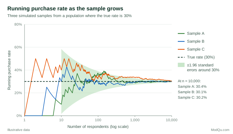
The shaded funnel shows the range within which about 95% of sample estimates fall at each sample size. Its width follows directly from the formula above:
| Respondents (n) | Standard error | Approximate 95% margin |
|---|---|---|
| 100 | 4.6 points | ±9.0 points |
| 400 | 2.3 points | ±4.5 points |
| 1,000 | 1.4 points | ±2.8 points |
| 4,000 | 0.7 points | ±1.4 points |
Moving from 100 to 400 respondents cuts the margin in half; moving from 1,000 to 4,000 buys only another 1.4 points.
What the law does not say
It does not say that luck "evens out"
The law works by dilution, not correction. If the first ten respondents happen to be unusually keen buyers, later respondents are not more likely to be reluctant. Their early surplus simply becomes a smaller and smaller fraction of a growing total. Believing otherwise is the gambler's fallacy, the expectation that chance will balance itself in the short run (Tversky & Kahneman, 1974).
It does not apply to small samples
Tversky and Kahneman (1971) found that even trained researchers expected small samples to resemble the population far more closely than probability allows, a bias they called belief in the "law of small numbers". In a related study, people judged that a small hospital and a large hospital were about equally likely to record days on which more than 60% of births were boys, although such days are much more common in the small one (Kahneman & Tversky, 1972). Business data show the same pattern. The best and worst performing stores, regions or sales representatives are often simply the smallest, because small units have the most variable averages (Wainer, 2007).
It does not remove bias
The law guarantees convergence to the mean of the process that generated the data, not to the mean of the population you care about. If a sample systematically over-represents some kinds of people, a larger sample converges, more and more precisely, to the wrong answer. Bethlehem (2010) shows that the selection bias of self-selected web surveys does not shrink as the sample grows. Meng (2018) formalises this "big data paradox": when the chance of responding is even slightly related to the answer, huge datasets can carry the information of a much smaller random sample. In a striking application, Bradley et al. (2021) found that one survey of about 250,000 respondents per week overestimated US COVID-19 vaccine uptake by 17 percentage points in May 2021, and that its accuracy was no better than that of a simple random sample of about 10 people.
Practical guidance for survey and business data
- Plan sample sizes with the square-root rule. Decide on the margin of error the decision needs, then calculate n. Beyond a certain point, extra respondents add cost faster than precision (Lohr, 2021).
- Plan for subgroups, not only the total. A 2,000-person survey split into 20 segments gives about 100 per segment and margins of up to about ±10 points for each.
- Spend on representativeness before size. Better sampling frames, follow-up of non-respondents and weighting usually do more for accuracy than doubling a biased sample. Response rates alone are a weak guide to nonresponse bias; what matters is whether responding is related to the survey answers (Groves & Peytcheva, 2008).
- Be cautious with ranked league tables. Before acting on the "top" or "bottom" unit, check its sample size and whether its result is outside the range expected from chance.
- Use finite-sample guarantees when stakes are high. Inequalities such as Hoeffding's (1963) give conservative bounds on how far an average of bounded values can stray at a given n, without assuming normality.
Common mistakes
- Treating a large n as proof of accuracy. Size controls random error only; it says nothing about coverage, nonresponse or measurement error.
- Comparing raw rates across groups of very different sizes without reporting standard errors.
- Stopping data collection when the result looks right. Watching a running average and stopping at a favourable moment builds early random swings into the final estimate.
- Forgetting the independence assumption. Clustered samples, repeated measures from the same customers or panel members, and correlated responses all reduce the effective sample size.
Key takeaways
The law of large numbers is the reason a well-drawn sample of a thousand people can describe a market of millions. Its practical form is the square-root rule: precision improves with √n, so gains slow quickly as samples grow. Small samples produce extreme results more often than intuition suggests, and large samples converge reliably only to the truth of the process that produced them. Good survey practice therefore pairs adequate sample sizes with careful attention to how respondents were selected.
References
Bernoulli, J. (2006). The art of conjecturing, together with Letter to a friend on sets in court tennis (E. D. Sylla, Trans.). Johns Hopkins University Press. (Original work published 1713)
Bethlehem, J. (2010). Selection bias in web surveys. International Statistical Review, 78(2), 161–188. https://doi.org/10.1111/j.1751-5823.2010.00112.x
Bradley, V. C., Kuriwaki, S., Isakov, M., Sejdinovic, D., Meng, X.-L., & Flaxman, S. (2021). Unrepresentative big surveys significantly overestimated US vaccine uptake. Nature, 600(7890), 695–700. https://doi.org/10.1038/s41586-021-04198-4
Groves, R. M., & Peytcheva, E. (2008). The impact of nonresponse rates on nonresponse bias: A meta-analysis. Public Opinion Quarterly, 72(2), 167–189. https://doi.org/10.1093/poq/nfn011
Hoeffding, W. (1963). Probability inequalities for sums of bounded random variables. Journal of the American Statistical Association, 58(301), 13–30. https://doi.org/10.1080/01621459.1963.10500830
Kahneman, D., & Tversky, A. (1972). Subjective probability: A judgment of representativeness. Cognitive Psychology, 3(3), 430–454. https://doi.org/10.1016/0010-0285(72)90016-3
Lohr, S. L. (2021). Sampling: Design and analysis (3rd ed.). Chapman and Hall/CRC. https://doi.org/10.1201/9780429298899
Meng, X.-L. (2018). Statistical paradises and paradoxes in big data (I): Law of large populations, big data paradox, and the 2016 US presidential election. The Annals of Applied Statistics, 12(2), 685–726. https://doi.org/10.1214/18-AOAS1161SF
Tversky, A., & Kahneman, D. (1971). Belief in the law of small numbers. Psychological Bulletin, 76(2), 105–110. https://doi.org/10.1037/h0031322
Tversky, A., & Kahneman, D. (1974). Judgment under uncertainty: Heuristics and biases. Science, 185(4157), 1124–1131. https://doi.org/10.1126/science.185.4157.1124
Wainer, H. (2007). The most dangerous equation. American Scientist, 95(3), 249. https://doi.org/10.1511/2007.65.1026
Wasserman, L. (2004). All of statistics: A concise course in statistical inference. Springer. https://doi.org/10.1007/978-0-387-21736-9