
Statistics · Causal inference
Targeted Maximum Likelihood Estimation for Causal Knowledge from Observational Data
How targeted maximum likelihood estimation combines an outcome model and a propensity score to estimate causal effects from observational data, with a worked survey example, assumptions and practical cautions.
Many business questions about cause and effect have to be answered without an experiment. Did attending a product webinar make customers more likely to buy? Did a loyalty programme raise retention? The people who took part chose to do so, and they differ from those who did not. Standard regression adjustment handles some of this, but it depends heavily on getting the model right. Targeted maximum likelihood estimation (TMLE), introduced by van der Laan and Rubin (2006), is a method designed to estimate a specific causal quantity as accurately as possible while allowing flexible, data-driven modelling. This article explains what TMLE does, why it is useful, and what it cannot fix.
The causal question
TMLE starts by defining the target precisely. In the potential outcomes framework, each customer has two possible outcomes: whether they would buy if they attended the webinar, and whether they would buy if they did not. Only one is observed (Rubin, 1974; Holland, 1986). The usual target is the average treatment effect (ATE): the difference in purchase rates if everyone attended versus if nobody did.
To estimate the ATE from observational data, three assumptions are needed (Hernán & Robins, 2020). Exchangeability requires that, once measured covariates are taken into account, attendees and non-attendees are comparable, so there is no unmeasured confounding. Positivity requires that every type of customer had some chance of both attending and not attending. Consistency requires that the treatment is well defined. TMLE relies on all three, like every other adjustment method. Its advantage is statistical, not a way around these assumptions.
Two routes to adjustment, and their weaknesses
There are two classic ways to adjust for covariates.
Outcome modelling (g-computation) fits a model for the outcome given treatment and covariates, predicts every person's outcome under attendance and under non-attendance, and averages the difference. It is efficient when the outcome model is correct, but biased when it is not.
Propensity score weighting models the probability of treatment given covariates, the propensity score (Rosenbaum & Rubin, 1983), and weights each person by the inverse of the probability of the treatment they actually received. It is unbiased when the propensity model is correct, but it can be unstable when some weights are very large.
Doubly robust estimators combine both models and remain consistent if either one is correctly specified (Robins et al., 1994; Bang & Robins, 2005). TMLE is a doubly robust estimator with some additional practical advantages.
How TMLE works
TMLE proceeds in four steps, shown in Figure 1 (Schuler & Rose, 2017; Luque-Fernandez et al., 2018).
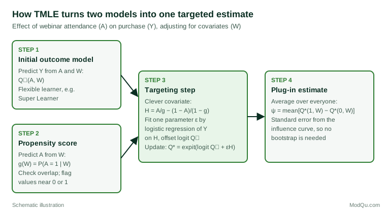
- Fit an initial outcome model. Estimate the probability of purchase given attendance and covariates, Q⁰(A, W). Because no particular model is assumed to be correct, a flexible approach is recommended. Super Learner, a cross-validated ensemble that combines several algorithms, such as regression, regularised regression and tree-based methods, is the usual choice (van der Laan et al., 2007).
- Fit a propensity score model. Estimate the probability of attendance given covariates, g(W), again flexibly.
- Target the initial estimate. The initial outcome model was built to predict well, not to estimate the ATE well, so it may carry bias for that specific target. TMLE corrects this with a small, targeted update that uses the propensity score.
- Compute the plug-in estimate. The ATE is the average of the updated predictions under attendance minus those under non-attendance, across the whole sample. Its standard error comes from the estimated influence curve, so confidence intervals require no bootstrap.
The update in step 3 uses a "clever covariate" built from the propensity score:
H(A, W) = A ÷ g(W) − (1 − A) ÷ (1 − g(W))
A one-parameter logistic regression of the outcome on H, with the initial predictions as an offset, gives a fluctuation parameter ε, and the predictions are updated:
logit Q*(A, W) = logit Q⁰(A, W) + ε × H(A, W)
ATE = (1 ÷ n) Σ [Q*(1, Wi) − Q*(0, Wi)]
If the initial outcome model was already unbiased for the ATE, ε will be close to zero and the update changes little. If it was not, the clever covariate shifts the predictions in the direction that removes the bias, using exactly the information in the propensity score that the outcome model missed. Because the update is tied to the efficient influence curve of the ATE, the resulting estimator is not only doubly robust but also efficient when both models are estimated well: among a broad class of estimators it has the smallest possible variance (van der Laan & Rose, 2011).
The targeting step is what distinguishes TMLE. It removes the bias in the initial estimate that matters for the chosen target, and the final estimate is a substitution (plug-in) estimator: it averages predicted probabilities, so a probability-scale estimate always respects the bounds of 0 and 1 (van der Laan & Rose, 2011). Some other doubly robust estimators can produce impossible values when propensity scores are extreme.
A worked example: webinar attendance and purchase
Suppose a hypothetical software company links a survey of 4,000 trial users to its sales records. Of these, 1,481 (37%) attended a product webinar. Covariates include company size, prior product use and a survey measure of purchase intent. The outcome is purchase within three months. The data were simulated so that the true effect of attendance is known to be 7.6 percentage points.
| Method | Estimated effect (points) | 95% CI |
|---|---|---|
| Unadjusted difference | 24.9 | 22.0 to 27.8 |
| Outcome regression (g-computation) | 8.3 | not computed |
| Inverse probability weighting | 7.5 | about 3.6 to 11.4 |
| TMLE | 7.3 | 4.3 to 10.2 |
Attendees bought at 43.2% and non-attendees at 18.3%, but most of that gap reflects who chose to attend: users with higher intent and heavier prior use. All three adjusted estimates fall close to the true effect. TMLE provides a confidence interval directly, from the influence curve, and its interval is narrower than that of weighting. In real data, the difference between methods is often larger, because outcome and propensity models are rarely correct and the flexible learners used in TMLE can reduce the resulting bias. These figures are illustrative.
Diagnostics and assumptions
- Check positivity. Inspect the distribution of propensity scores among attendees and non-attendees. Scores near 0 or 1 signal customer types who almost always or almost never attend, and estimates for them rely on extrapolation. Petersen et al. (2012) describe how to diagnose such violations and the options for responding, including truncating scores and redefining the target population. Truncation trades a little bias for much lower variance and should be reported.
- Use cross-validation for the learners. Flexible learners can overfit. Super Learner's cross-validation, or sample splitting as in double/debiased machine learning (Chernozhukov et al., 2018), protects the inference.
- Remember what double robustness does not do. Kang and Schafer (2007) showed that when both models are moderately wrong and some weights are large, doubly robust estimators can perform worse than simpler methods. Double robustness is protection against one model being wrong, not against both.
- Unmeasured confounding remains. No estimator removes bias from confounders that were not measured. Pair TMLE with a sensitivity analysis.
Practical guidance for survey and business data
- Define the estimand first. Decide whether the question concerns everyone (the ATE) or only those who were treated (the average effect among the treated), since TMLE can target either.
- Measure confounders before treatment. Survey items used as covariates must describe customers before they attended. Attitudes measured afterwards may themselves be affected by the webinar.
- Use established software. The tmle package for R implements the method with Super Learner and influence-curve inference (Gruber & van der Laan, 2012).
- Account for survey design. When data come from a weighted sample, incorporate the weights and report how they were used.
- Report all the ingredients. State the covariates, the algorithms included in the Super Learner library, any truncation of propensity scores, and the distribution of scores in each group, so that others can judge the analysis.
Common mistakes
- Treating TMLE as a cure for confounding. It improves estimation given the measured covariates; it does not make an observational comparison equivalent to a randomised experiment.
- Adjusting for variables affected by the treatment. Including post-treatment variables, such as satisfaction measured after the webinar, can block part of the effect or introduce bias.
- Ignoring extreme propensity scores. A precise-looking interval can hide heavy reliance on a handful of customers with very unusual treatment probabilities.
Key takeaways
TMLE estimates a clearly defined causal effect by combining an outcome model and a propensity score model, then applying a targeted update that removes bias for the specific quantity of interest. It is doubly robust, works well with machine learning methods such as Super Learner, keeps estimates within valid bounds and provides standard errors without resampling. It does not relax the core assumptions of causal inference: measured confounders, adequate overlap and a well-defined treatment are still essential, and a sensitivity analysis for unmeasured confounding remains good practice.
References
Bang, H., & Robins, J. M. (2005). Doubly robust estimation in missing data and causal inference models. Biometrics, 61(4), 962–973. https://doi.org/10.1111/j.1541-0420.2005.00377.x
Chernozhukov, V., Chetverikov, D., Demirer, M., Duflo, E., Hansen, C., Newey, W., & Robins, J. (2018). Double/debiased machine learning for treatment and structural parameters. The Econometrics Journal, 21(1), C1–C68. https://doi.org/10.1111/ectj.12097
Gruber, S., & van der Laan, M. J. (2012). tmle: An R package for targeted maximum likelihood estimation. Journal of Statistical Software, 51(13), 1–35. https://doi.org/10.18637/jss.v051.i13
Hernán, M. A., & Robins, J. M. (2020). Causal inference: What if. Chapman & Hall/CRC.
Holland, P. W. (1986). Statistics and causal inference. Journal of the American Statistical Association, 81(396), 945–960. https://doi.org/10.1080/01621459.1986.10478354
Kang, J. D. Y., & Schafer, J. L. (2007). Demystifying double robustness: A comparison of alternative strategies for estimating a population mean from incomplete data. Statistical Science, 22(4), 523–539. https://doi.org/10.1214/07-STS227
Luque-Fernandez, M. A., Schomaker, M., Rachet, B., & Schnitzer, M. E. (2018). Targeted maximum likelihood estimation for a binary treatment: A tutorial. Statistics in Medicine, 37(16), 2530–2546. https://doi.org/10.1002/sim.7628
Petersen, M. L., Porter, K. E., Gruber, S., Wang, Y., & van der Laan, M. J. (2012). Diagnosing and responding to violations in the positivity assumption. Statistical Methods in Medical Research, 21(1), 31–54. https://doi.org/10.1177/0962280210386207
Robins, J. M., Rotnitzky, A., & Zhao, L. P. (1994). Estimation of regression coefficients when some regressors are not always observed. Journal of the American Statistical Association, 89(427), 846–866. https://doi.org/10.1080/01621459.1994.10476818
Rosenbaum, P. R., & Rubin, D. B. (1983). The central role of the propensity score in observational studies for causal effects. Biometrika, 70(1), 41–55. https://doi.org/10.1093/biomet/70.1.41
Rubin, D. B. (1974). Estimating causal effects of treatments in randomized and nonrandomized studies. Journal of Educational Psychology, 66(5), 688–701. https://doi.org/10.1037/h0037350
Schuler, M. S., & Rose, S. (2017). Targeted maximum likelihood estimation for causal inference in observational studies. American Journal of Epidemiology, 185(1), 65–73. https://doi.org/10.1093/aje/kww165
van der Laan, M. J., Polley, E. C., & Hubbard, A. E. (2007). Super learner. Statistical Applications in Genetics and Molecular Biology, 6(1), Article 25. https://doi.org/10.2202/1544-6115.1309
van der Laan, M. J., & Rose, S. (2011). Targeted learning: Causal inference for observational and experimental data. Springer. https://doi.org/10.1007/978-1-4419-9782-1
van der Laan, M. J., & Rubin, D. (2006). Targeted maximum likelihood learning. The International Journal of Biostatistics, 2(1), Article 11. https://doi.org/10.2202/1557-4679.1043