
Statistics · Causal inference
Sensitivity Analysis for Unmeasured Confounding in Causal Knowledge
How sensitivity analysis asks how strong an unmeasured confounder would have to be to overturn an observational finding, with E-values, partial R² methods, a worked churn example and reporting guidance.
Most causal questions in business are answered with observational data. A company wants to know whether customers who use its mobile app are less likely to cancel, whether a loyalty scheme raises spending, or whether staff who complete a training course perform better. Nobody was randomly assigned to use the app or take the course, so the people who did may differ from those who did not in ways that also affect the outcome. Analysts adjust for the differences they can measure, but every observational estimate rests on an assumption that cannot be tested from the data: that no important confounding variable has been left out.
Sensitivity analysis for unmeasured confounding does not try to prove that assumption. Instead, it asks a quantitative question: how strong would an unmeasured confounder have to be to change the conclusion? If the answer is "implausibly strong", the finding is robust. If the answer is "about as strong as variables we already know matter", the finding is fragile and should be reported as such.
Why adjustment is never the whole story
In the potential outcomes framework, a causal effect compares the outcome a unit would have with the treatment and without it, only one of which is ever observed (Holland, 1986). Observational studies estimate the missing outcomes from other units, and this works only if treated and untreated units are comparable once measured covariates are taken into account. In the language of causal diagrams, all "back-door" paths between treatment and outcome must be blocked by the adjustment set (Pearl, 2009).
No analyst can confirm that this condition holds. Customers who adopt an app may be more engaged with the brand, more digitally confident, or more satisfied to begin with, and a customer database or survey rarely measures all of these well. Leamer (1983) argued that empirical conclusions deserve belief only when they survive reasonable changes in the assumptions behind them. Sensitivity analysis applies that principle to the assumption of no unmeasured confounding, and Rosenbaum (2002) treats it as an essential part of any observational study.
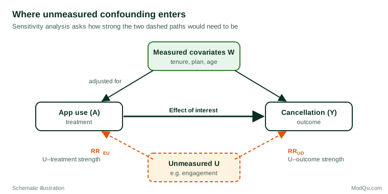
Figure 1 shows the structure. Measured covariates such as tenure, plan and age are adjusted for. An unmeasured variable U that affects both app use and cancellation opens a path that adjustment cannot block. Sensitivity analysis characterises U by the strength of its two arrows.
A brief history: from smoking to E-values
The idea is older than modern causal inference. In the 1950s, critics of the link between smoking and lung cancer suggested that a hidden genetic factor might cause both. Cornfield et al. (1959) showed that for such a factor to explain away the roughly ninefold higher risk among heavy smokers, it would have to be at least nine times as common among smokers as among non-smokers, which was implausible. This reasoning, now called the Cornfield inequality, established the core logic: weak associations can be explained by modest confounding, but strong associations require confounders of matching strength.
Rosenbaum and Rubin (1983) formalised the approach for a binary unmeasured covariate. The analyst specifies its prevalence among treated and untreated units and its association with the outcome, and recalculates the effect under each scenario. Later work generalised these bias formulas to continuous outcomes and confounders of any type (Lin et al., 1998; VanderWeele & Arah, 2011).
Main families of sensitivity analysis
Bias formulas and the E-value
Ding and VanderWeele (2016) showed that, for a risk ratio, the maximum bias an unmeasured confounder can produce depends on two quantities: RREU, the strength of its association with the treatment, and RRUD, the strength of its association with the outcome. The bias factor is:
B = (RREU × RRUD) ÷ (RREU + RRUD − 1)
An observed risk ratio can be fully explained away only if B is at least as large as the observed ratio. VanderWeele and Ding (2017) summarised this in a single number, the E-value: the minimum strength of association, on the risk ratio scale, that an unmeasured confounder would need with both the treatment and the outcome to move the estimate to the null. For a risk ratio RR above 1:
E-value = RR + √(RR × (RR − 1))
For a protective risk ratio below 1, the formula is applied to its reciprocal. An E-value is also reported for the confidence limit closest to the null, which shows how much confounding would be needed to make the result compatible with no effect. The E-value needs no assumptions about the confounder's prevalence, so it can be calculated for almost any published estimate.
Partial R² and the robustness value
For linear regression estimates, Cinelli and Hazlett (2020) express sensitivity in terms of how much residual variance an unmeasured confounder would explain in the treatment and in the outcome, measured by partial R² values. Their robustness value is the share of residual variance that a confounder would need to explain in both treatment and outcome to reduce the estimate to zero, or to make it statistically insignificant. A key strength of the framework is formal benchmarking: the analyst can ask what would happen if the unmeasured confounder were, for instance, as strong as the strongest measured covariate, or three times as strong. Frank (2000) developed a related threshold based on correlations, and Imbens (2003) proposed calibrating a binary unmeasured confounder against the explanatory power of observed covariates.
Coefficient stability
Economists often reason from how much an estimate moves when observed controls are added. Altonji et al. (2005) argued that selection on observed variables can serve as a guide to selection on unobserved ones. Oster (2019) showed that coefficient movement alone is uninformative unless it is scaled by the change in R², and proposed a parameter, δ, measuring how strong selection on unobservables would have to be, relative to observables, to drive the effect to zero. Values of δ above 1 are commonly read as evidence of robustness, though the result depends on the assumed maximum achievable R².
Design-based bounds
In matched studies, Rosenbaum (2002) uses a parameter Γ that bounds how much the odds of treatment can differ between two units that look identical on measured covariates. At Γ = 1 there is no hidden bias; at Γ = 2 one unit could be twice as likely to be treated as its match. The analyst reports the largest Γ at which the conclusion still holds.
Probabilistic bias analysis and external adjustment
Analysts can also place probability distributions on the bias parameters and simulate corrected estimates (Greenland, 1996; Lash et al., 2009). When information about the confounder is available from another source, such as a validation subsample in which it was measured, it can be used for external adjustment (Schneeweiss, 2006). This is a natural fit for survey research: a short follow-up survey of a subsample can measure the suspected confounder directly.
A worked example: app use and cancellation
Suppose a hypothetical subscription business links a survey of 3,000 customers to its records of who cancelled over the following twelve months. After adjusting for tenure, plan type, age group, region and prior complaints, customers who regularly used the mobile app had a risk ratio for cancellation of 0.60 (95% CI 0.46 to 0.78) compared with non-users. Taken at face value, app use reduces cancellation by 40%.
Because the risk ratio is below 1, the E-value is calculated from its reciprocal, 1 ÷ 0.60 = 1.67:
E-value = 1.67 + √(1.67 × 0.67) ≈ 2.72
For the upper confidence limit, 1 ÷ 0.78 = 1.28, giving an E-value of about 1.88. In words: an unmeasured confounder associated with both app use and cancellation by a risk ratio of 2.72 each, above and beyond the measured covariates, could explain away the estimated effect. A confounder associated with both by 1.88 could make the result compatible with no effect. Weaker confounding could not do either.
The E-value is the point on the diagonal, but many other combinations produce the same bias. Figure 2 shows the full curve. A confounder twice as common among app users (RREU = 2) would need to raise the risk of cancellation fivefold (RRUD = 5) to explain away the point estimate.
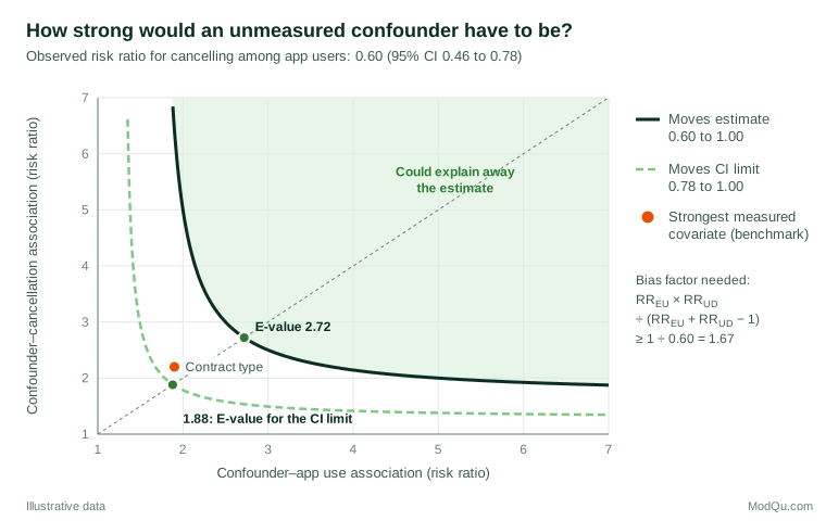
Is that plausible? The numbers need context, so the analyst benchmarks them against measured variables. Suppose that the strongest measured confounder, contract type, has associations of about 1.9 with app use and 2.2 with cancellation. Its bias factor is (1.9 × 2.2) ÷ (1.9 + 2.2 − 1) ≈ 1.35. An unmeasured confounder as strong as contract type could therefore push the confidence interval to include 1, but it could not remove the whole effect. The honest conclusion is that app use is probably associated with lower cancellation even after allowing for plausible hidden confounding, but the size of the effect is uncertain and could be considerably smaller than 40%. If unmeasured engagement is believed to be stronger than contract type, it should be measured before the estimate drives major investment.
The risk ratio here was estimated directly. When an outcome is common and only an odds ratio is available, VanderWeele and Ding (2017) suggest approximating the risk ratio by the square root of the odds ratio before computing the E-value. And the benchmarking above is informal: Cinelli and Hazlett (2020) caution that the observed strength of a covariate, measured after adjustment for the others, is not always a valid bound on what a similar unmeasured variable could do, and their formal bounds are preferable for linear models.
Interpreting results responsibly
Sensitivity analysis is easy to misuse. Ioannidis et al. (2019) note that E-values are often reported without any discussion of which confounders might plausibly reach the threshold, and that a large E-value can create false reassurance when the study has other problems such as selection bias or measurement error. Some practical rules follow:
- Name candidate confounders. A sensitivity result is useful only when it is compared with specific variables that could plausibly be missing.
- Use benchmarks. Compare the required strength with the strength of measured covariates, or with associations reported in other studies.
- Report the confidence limit as well as the point estimate. Explaining away statistical significance usually needs much weaker confounding than explaining away the whole effect.
- Remember other biases. Unmeasured confounding is only one threat. Selection into the survey, nonresponse, measurement error in self-reported behaviour and reverse causation can all matter as much.
- Triangulate. Conclusions are strongest when different designs with different sources of bias point in the same direction (Lawlor et al., 2016).
Practical guidance for survey and business data
- Plan for sensitivity analysis at the design stage. List the confounders that might matter, measure as many as possible, and collect at least a rough measure of those that are hard to capture, such as attitudes, engagement or prior intentions.
- Use the survey to fill the gaps. Customer records lack attitudes and motives; surveys can capture them. A linked survey can turn an unmeasured confounder into a measured one, or at least provide external information for adjustment.
- Present the result in plain language. "A hidden factor would need to make app users nearly three times as likely to stay, and also be nearly three times as common among them, to explain this away" is clearer for decision-makers than a bare number.
Common mistakes
- Treating a large E-value as proof of causation. It shows robustness to one specific kind of bias, under the assumptions of the method.
- Ignoring that the confounder must act beyond measured covariates. The required associations are conditional on the variables already adjusted for, which makes informal comparison with unadjusted correlations misleading.
Key takeaways
Every causal estimate from observational data depends on the untestable assumption that no important confounder is missing. Sensitivity analysis replaces a yes-or-no debate about that assumption with a quantitative statement of how strong hidden confounding would need to be to change the conclusion. E-values, partial R² methods, coefficient stability, Rosenbaum bounds and probabilistic bias analysis each answer that question for different models and designs. Their value depends on interpretation: name plausible confounders, benchmark against measured variables, report results for both the estimate and its confidence limit, and use surveys to measure the confounders that records miss.
References
Altonji, J. G., Elder, T. E., & Taber, C. R. (2005). Selection on observed and unobserved variables: Assessing the effectiveness of Catholic schools. Journal of Political Economy, 113(1), 151–184. https://doi.org/10.1086/426036
Cinelli, C., & Hazlett, C. (2020). Making sense of sensitivity: Extending omitted variable bias. Journal of the Royal Statistical Society Series B: Statistical Methodology, 82(1), 39–67. https://doi.org/10.1111/rssb.12348
Cornfield, J., Haenszel, W., Hammond, E. C., Lilienfeld, A. M., Shimkin, M. B., & Wynder, E. L. (1959). Smoking and lung cancer: Recent evidence and a discussion of some questions. Journal of the National Cancer Institute, 22(1), 173–203. https://doi.org/10.1093/jnci/22.1.173
Ding, P., & VanderWeele, T. J. (2016). Sensitivity analysis without assumptions. Epidemiology, 27(3), 368–377. https://doi.org/10.1097/EDE.0000000000000457
Frank, K. A. (2000). Impact of a confounding variable on a regression coefficient. Sociological Methods & Research, 29(2), 147–194. https://doi.org/10.1177/0049124100029002001
Greenland, S. (1996). Basic methods for sensitivity analysis of biases. International Journal of Epidemiology, 25(6), 1107–1116. https://doi.org/10.1093/ije/25.6.1107
Holland, P. W. (1986). Statistics and causal inference. Journal of the American Statistical Association, 81(396), 945–960. https://doi.org/10.1080/01621459.1986.10478354
Imbens, G. W. (2003). Sensitivity to exogeneity assumptions in program evaluation. American Economic Review, 93(2), 126–132. https://doi.org/10.1257/000282803321946921
Ioannidis, J. P. A., Tan, Y. J., & Blum, M. R. (2019). Limitations and misinterpretations of E-values for sensitivity analyses of observational studies. Annals of Internal Medicine, 170(2), 108–111. https://doi.org/10.7326/M18-2159
Lash, T. L., Fox, M. P., & Fink, A. K. (2009). Applying quantitative bias analysis to epidemiologic data. Springer. https://doi.org/10.1007/978-0-387-87959-8
Lawlor, D. A., Tilling, K., & Davey Smith, G. (2016). Triangulation in aetiological epidemiology. International Journal of Epidemiology, 45(6), 1866–1886. https://doi.org/10.1093/ije/dyw314
Leamer, E. E. (1983). Let's take the con out of econometrics. The American Economic Review, 73(1), 31–43.
Lin, D. Y., Psaty, B. M., & Kronmal, R. A. (1998). Assessing the sensitivity of regression results to unmeasured confounders in observational studies. Biometrics, 54(3), 948–963. https://doi.org/10.2307/2533848
Oster, E. (2019). Unobservable selection and coefficient stability: Theory and evidence. Journal of Business & Economic Statistics, 37(2), 187–204. https://doi.org/10.1080/07350015.2016.1227711
Pearl, J. (2009). Causality: Models, reasoning, and inference (2nd ed.). Cambridge University Press. https://doi.org/10.1017/CBO9780511803161
Rosenbaum, P. R. (2002). Observational studies (2nd ed.). Springer. https://doi.org/10.1007/978-1-4757-3692-2
Rosenbaum, P. R., & Rubin, D. B. (1983). Assessing sensitivity to an unobserved binary covariate in an observational study with binary outcome. Journal of the Royal Statistical Society Series B: Statistical Methodology, 45(2), 212–218. https://doi.org/10.1111/j.2517-6161.1983.tb01242.x
Schneeweiss, S. (2006). Sensitivity analysis and external adjustment for unmeasured confounders in epidemiologic database studies of therapeutics. Pharmacoepidemiology and Drug Safety, 15(5), 291–303. https://doi.org/10.1002/pds.1200
VanderWeele, T. J., & Arah, O. A. (2011). Bias formulas for sensitivity analysis of unmeasured confounding for general outcomes, treatments, and confounders. Epidemiology, 22(1), 42–52. https://doi.org/10.1097/EDE.0b013e3181f74493
VanderWeele, T. J., & Ding, P. (2017). Sensitivity analysis in observational research: Introducing the E-value. Annals of Internal Medicine, 167(4), 268–274. https://doi.org/10.7326/M16-2607