
Statistics · Causal inference
Causal Forests and Heterogeneous Treatment Effect Estimation
How causal forests adapt random forests to estimate how a treatment effect varies from customer to customer, why honest estimation matters for valid intervals, and how to use the results for targeting.
A retention offer raises renewal by two percentage points on average. That single number answers one question well: was the campaign worth running for everyone? It answers a more useful question badly: who should receive the offer next time? If the offer works strongly for new customers and not at all for long-standing ones, sending it to everyone wastes budget, and sending it to the customers who are most likely to leave may waste even more. Questions of this kind are about heterogeneous treatment effects: the way the causal effect of an action varies with the characteristics of the person, store or region that receives it.
The causal forest is one of the most widely used tools for estimating such variation. Introduced by Wager and Athey (2018) and generalised by Athey et al. (2019), it adapts the random forest, a flexible prediction method, so that it estimates treatment effects rather than outcomes, and does so in a way that supports confidence intervals. This article explains the idea, walks through a worked example and sets out the practical checks that keep the method honest.
From average effects to conditional effects
Causal questions are clearest in the language of potential outcomes (Rubin, 1974; Imbens & Rubin, 2015). Each customer i has an outcome Yi(1) if treated, for example if sent the offer, and Yi(0) if not. The individual effect is the difference between the two, but only one of them is ever observed. The other is the counterfactual.
Because individual effects cannot be seen, analysts estimate averages. The average treatment effect (ATE) averages over everyone. The conditional average treatment effect (CATE) averages over everyone who shares a set of characteristics x, such as tenure, plan type and region:
τ(x) = E[Y(1) − Y(0) | X = x]
The CATE is the target of a causal forest. It is not the individual effect, which remains unknowable, but it is the best available guide to how a person with characteristics x would respond on average.
Two assumptions are needed to estimate τ(x) from data. In a randomised experiment both hold by design. In observational data they must be argued:
- Unconfoundedness. Given the measured covariates, treatment is unrelated to the potential outcomes, so there is no unmeasured confounding (Rosenbaum & Rubin, 1983).
- Overlap. Every type of customer has some chance of being treated and some chance of not being treated. Where overlap fails, no method can estimate the effect without extrapolating.
Why simple subgroup analysis falls short
The traditional approach is to split the sample by a few variables chosen in advance, such as age band or region, and compare effects. This is transparent but limited. It finds only the heterogeneity the analyst thought to look for, it handles interactions between variables poorly, and it invites a familiar abuse: slicing the data many ways and reporting the subgroup where the effect looks largest. Guidance on subgroup reporting in clinical trials warns that unplanned subgroup findings are often false positives and recommends prespecification and formal tests of interaction (Wang et al., 2007).
Machine learning offers a way to search across many covariates at once. The danger is that a flexible algorithm left to search freely will also find patterns in noise. The contribution of causal trees and forests is a search procedure combined with safeguards that keep the resulting estimates and intervals valid (Athey & Imbens, 2016, 2019).
From regression trees to causal trees
A regression tree splits the data recursively into groups that are as different as possible in their average outcome (Breiman et al., 1984). A causal tree keeps the splitting machinery but changes the goal: it looks for splits that separate customers whose treatment effects differ. Within each final group, or leaf, the effect is estimated as the difference between the mean outcome of treated and untreated customers in that leaf.
Athey and Imbens (2016) showed that this naive version is biased, because the same data are used to choose the splits and to estimate the effects. A split chosen because the treated customers on one side happened to do unusually well will overstate the effect in that leaf. Their remedy is honest estimation.
Honest estimation
An honest tree divides the sample in two. One half is used only to decide where to split. The other half, which played no part in building the tree, is used only to estimate the effect in each leaf. Because the estimation sample is independent of the choice of leaves, the leaf estimates behave like estimates from a prespecified subgroup analysis, and ordinary confidence intervals are valid. The price is precision: each step uses only part of the data. Athey and Imbens (2016) also modified the splitting criterion so that it rewards splits that reveal genuine differences in effects while penalising splits that would make the leaf estimates too noisy.
Causal forests
A single tree is unstable: a small change in the data can produce a very different tree. Random forests address this by averaging many trees, each grown on a random subsample with a random subset of variables considered at each split (Breiman, 2001). A causal forest does the same with honest causal trees.
The prediction for a new customer with characteristics x can be read as a weighted comparison of treated and untreated customers in the training data. Customers who often share a leaf with x across the trees receive large weights; customers who rarely do receive small ones. Athey et al. (2019) made this view formal: a generalised random forest uses the trees only to find these adaptive weights, then solves a local estimating equation, here a weighted comparison of treated and untreated outcomes, at each point x.
Wager and Athey (2018) proved that, with honest trees grown on subsamples, causal forest estimates are consistent and approximately normally distributed, and that their variance can be estimated. This is what separates the method from many earlier machine learning approaches: it delivers an estimate of τ(x) together with a confidence interval.
Orthogonalisation in observational data
When treatment is not randomised, splits can pick up differences in who was treated rather than differences in effects. Generalised random forests reduce this risk through local centring (Athey et al., 2019). Before the forest is grown, two auxiliary models are fitted: one predicts the outcome from the covariates, and one predicts the probability of treatment, the propensity score. The forest then works with residuals, the outcome minus its prediction and the treatment minus its predicted probability. The idea goes back to Robinson's (1988) partially linear model and is the same residual-on-residual logic used in double machine learning (Chernozhukov et al., 2018). Nie and Wager (2021) developed it into a general recipe, the R-learner, which can be combined with any flexible learner.
Orthogonalisation reduces sensitivity to errors in the auxiliary models. It does not remove bias from confounders that were never measured.
A worked example
Consider a hypothetical subscription business that randomises a retention discount among 8,000 customers approaching renewal. Half receive the offer. The overall renewal rate rises from 78% in the control group to 80% in the treated group, an average effect of about 2 percentage points. The covariates include tenure, monthly spend, number of support contacts in the last quarter, plan type and satisfaction from the most recent survey.
A causal forest fitted to these illustrative data suggests that the effect depends mainly on tenure. Figure 1 shows the estimated CATE against tenure, holding the other covariates at typical values.
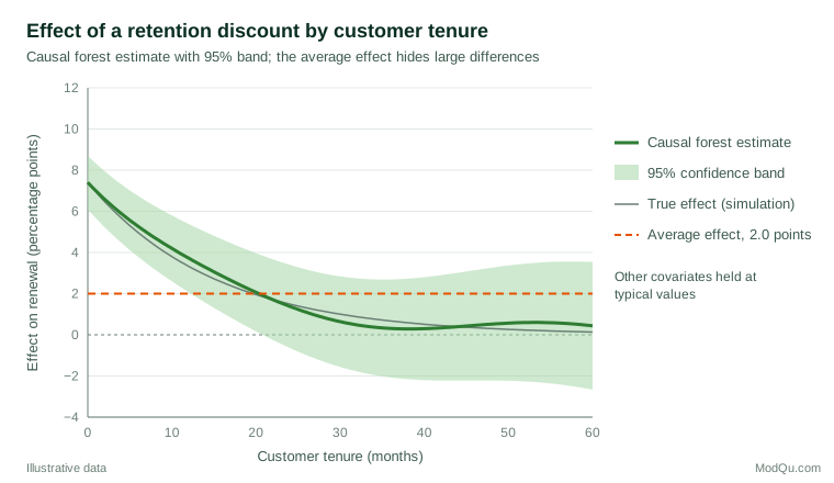
The average of 2 points hides a striking pattern. Customers in their first few months respond strongly, by around 6 to 7 points, while customers with more than three years of tenure barely respond at all. The confidence band widens at high tenure because fewer customers in the illustrative data have been with the firm that long.
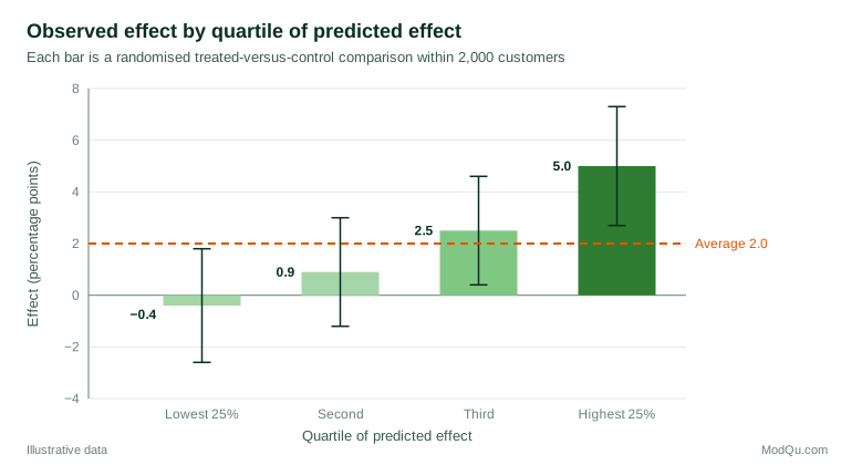
A pointwise curve is a useful picture, but it should not be the main evidence that heterogeneity exists. A more robust check sorts customers into groups by their predicted effect, using predictions made without each customer's own data, and then estimates the actual average effect within each group from the experiment. Table 1 shows the result for the hypothetical study.
| Quartile of predicted effect | Customers | Estimated effect (points) | 95% interval |
|---|---|---|---|
| Lowest 25% | 2,000 | −0.4 | −2.6 to 1.8 |
| Second | 2,000 | 0.9 | −1.2 to 3.0 |
| Third | 2,000 | 2.5 | 0.4 to 4.6 |
| Highest 25% | 2,000 | 5.0 | 2.7 to 7.3 |
Figure 2 displays the same estimates. Because each group's effect is estimated by a simple comparison of randomised treated and control customers, it does not rely on the forest being right in detail. If the forest had found only noise, the four bars would be roughly level.
From estimates to decisions
The practical value of heterogeneous effects lies in targeting. In the example, offering the discount only to the top half of predicted responders would capture most of the campaign's gain at half the cost. Ascarza (2018) reported field experiments in which targeting retention efforts at the customers judged most likely to churn was less effective than targeting the customers most responsive to the intervention, because high risk and high responsiveness are not the same thing. A causal forest estimates responsiveness directly.
Turning estimates into a rule is itself a statistical problem. Methods for learning treatment rules choose the policy that maximises expected benefit, subject to budget or fairness constraints, and quantify how much better it is than treating everyone or no one (Kitagawa & Tetenov, 2018; Athey & Wager, 2021). A sound workflow evaluates any proposed rule on data that were not used to build it, and ideally in a fresh experiment.
Alternatives and relatives
Causal forests are one member of a larger family. Meta-learners combine standard prediction models in different ways: the T-learner fits separate outcome models for treated and untreated customers and subtracts them, the S-learner includes treatment as one more input, and the X-learner uses each group's model to impute effects for the other, which helps when one group is much smaller (Künzel et al., 2019). The R-learner rests on the residual-on-residual idea described above (Nie & Wager, 2021).
Bayesian additive regression trees (BART) offer another route, with uncertainty that comes from the posterior distribution (Hill, 2011). Bayesian causal forests extend BART by modelling the untreated outcome and the treatment effect separately and including the estimated propensity score as a covariate, which reduces a form of bias caused by regularisation in observational data (Hahn et al., 2020). In a large data analysis competition, flexible methods of these kinds generally performed well in estimating effects from simulated observational data, although no method won in every setting (Dorie et al., 2019). Earlier work on randomised programme evaluations used sparse regression methods to identify which covariates modify an effect (Imai & Ratkovic, 2013).
No single method dominates. In practice, comparing two or three methods and checking whether they agree on which customers respond most is more informative than trusting any one of them.
Practical guidance for survey and business data
- Prefer randomised data where possible. Heterogeneity is hard to estimate even in experiments. With observational data, every bias that affects the average effect also affects the conditional effects, and often more severely.
- Plan for a large sample. Detecting differences in effects needs far more data than detecting an average effect, because each comparison uses only part of the sample. Effects estimated for a few thousand customers will usually be imprecise.
- Use pre-treatment covariates only. Satisfaction measured after the offer, or any variable the treatment could change, must not be used to define groups.
- Test before you interpret. Check whether the predicted effects actually sort customers by their observed effects, as in Table 1, before discussing which variables matter. Davis and Heller (2017) used causal forests on a randomised summer jobs programme and illustrate how forest predictions can be checked against held-out outcomes.
- Report variable importance cautiously. Forests report how often each variable is used for splitting. Frequent use does not mean the variable causes the difference; it may simply be correlated with the variable that does.
- Account for survey design. When the data come from a weighted survey or panel, weighted estimates and design-aware uncertainty matter for the final group effects just as for any other estimate.
Common mistakes
- Treating CATE estimates as individual effects. A predicted effect of 6 points for a customer is an estimate for people like that customer, not a statement about that person.
- Reading the curve without the interval. Pointwise intervals are wide in sparse regions. A dramatic shape at the edge of the data is often noise.
- Searching freely, then reporting the best subgroup. Honest estimation protects the forest's own estimates, not the analyst's choices made after looking at many outputs.
- Assuming orthogonalisation fixes confounding. It helps with model error in measured confounders, not with confounders that were never measured.
- Confusing prediction with persuasion. Customers most likely to churn, buy or click are not necessarily those whose behaviour the treatment changes.
Key takeaways
Causal forests estimate how a treatment effect varies with observed characteristics, using honest trees and averaging to produce estimates with valid confidence intervals. They work best with randomised data, large samples and pre-treatment covariates. Their real value comes from targeting: identifying where an action makes a difference. Validate heterogeneity with held-out group comparisons, treat individual predictions as averages for similar customers, and test any targeting rule before relying on it.
References
Ascarza, E. (2018). Retention futility: Targeting high-risk customers might be ineffective. Journal of Marketing Research, 55(1), 80–98. https://doi.org/10.1509/jmr.16.0163
Athey, S., & Imbens, G. (2016). Recursive partitioning for heterogeneous causal effects. Proceedings of the National Academy of Sciences, 113(27), 7353–7360. https://doi.org/10.1073/pnas.1510489113
Athey, S., & Imbens, G. W. (2019). Machine learning methods that economists should know about. Annual Review of Economics, 11, 685–725. https://doi.org/10.1146/annurev-economics-080217-053433
Athey, S., Tibshirani, J., & Wager, S. (2019). Generalized random forests. The Annals of Statistics, 47(2), 1148–1178. https://doi.org/10.1214/18-AOS1709
Athey, S., & Wager, S. (2021). Policy learning with observational data. Econometrica, 89(1), 133–161. https://doi.org/10.3982/ECTA15732
Breiman, L. (2001). Random forests. Machine Learning, 45(1), 5–32. https://doi.org/10.1023/A:1010933404324
Breiman, L., Friedman, J. H., Olshen, R. A., & Stone, C. J. (1984). Classification and regression trees. Wadsworth.
Chernozhukov, V., Chetverikov, D., Demirer, M., Duflo, E., Hansen, C., Newey, W., & Robins, J. (2018). Double/debiased machine learning for treatment and structural parameters. The Econometrics Journal, 21(1), C1–C68. https://doi.org/10.1111/ectj.12097
Davis, J. M. V., & Heller, S. B. (2017). Using causal forests to predict treatment heterogeneity: An application to summer jobs. American Economic Review, 107(5), 546–550. https://doi.org/10.1257/aer.p20171000
Dorie, V., Hill, J., Shalit, U., Scott, M., & Cervone, D. (2019). Automated versus do-it-yourself methods for causal inference: Lessons learned from a data analysis competition. Statistical Science, 34(1), 43–68. https://doi.org/10.1214/18-STS667
Hahn, P. R., Murray, J. S., & Carvalho, C. M. (2020). Bayesian regression tree models for causal inference: Regularization, confounding, and heterogeneous effects (with discussion). Bayesian Analysis, 15(3), 965–1056. https://doi.org/10.1214/19-BA1195
Hill, J. L. (2011). Bayesian nonparametric modeling for causal inference. Journal of Computational and Graphical Statistics, 20(1), 217–240. https://doi.org/10.1198/jcgs.2010.08162
Imai, K., & Ratkovic, M. (2013). Estimating treatment effect heterogeneity in randomized program evaluation. The Annals of Applied Statistics, 7(1), 443–470. https://doi.org/10.1214/12-AOAS593
Imbens, G. W., & Rubin, D. B. (2015). Causal inference for statistics, social, and biomedical sciences: An introduction. Cambridge University Press. https://doi.org/10.1017/CBO9781139025751
Kitagawa, T., & Tetenov, A. (2018). Who should be treated? Empirical welfare maximization methods for treatment choice. Econometrica, 86(2), 591–616. https://doi.org/10.3982/ECTA13288
Künzel, S. R., Sekhon, J. S., Bickel, P. J., & Yu, B. (2019). Metalearners for estimating heterogeneous treatment effects using machine learning. Proceedings of the National Academy of Sciences, 116(10), 4156–4165. https://doi.org/10.1073/pnas.1804597116
Nie, X., & Wager, S. (2021). Quasi-oracle estimation of heterogeneous treatment effects. Biometrika, 108(2), 299–319. https://doi.org/10.1093/biomet/asaa076
Robinson, P. M. (1988). Root-N-consistent semiparametric regression. Econometrica, 56(4), 931–954. https://doi.org/10.2307/1912705
Rosenbaum, P. R., & Rubin, D. B. (1983). The central role of the propensity score in observational studies for causal effects. Biometrika, 70(1), 41–55. https://doi.org/10.1093/biomet/70.1.41
Rubin, D. B. (1974). Estimating causal effects of treatments in randomized and nonrandomized studies. Journal of Educational Psychology, 66(5), 688–701. https://doi.org/10.1037/h0037350
Wager, S., & Athey, S. (2018). Estimation and inference of heterogeneous treatment effects using random forests. Journal of the American Statistical Association, 113(523), 1228–1242. https://doi.org/10.1080/01621459.2017.1319839
Wang, R., Lagakos, S. W., Ware, J. H., Hunter, D. J., & Drazen, J. M. (2007). Statistics in medicine: Reporting of subgroup analyses in clinical trials. New England Journal of Medicine, 357(21), 2189–2194. https://doi.org/10.1056/NEJMsr077003