
Statistics · Causal inference
Interrupted Time-Series Designs for Intervention Knowledge Evaluation
How interrupted time-series designs use repeated measurements before and after a launch, policy or price change to estimate its effect, with segmented regression, a worked tracker example and the main pitfalls.
Organisations change things all the time: a price rise, a new loyalty programme, a rebrand, a change to the returns policy, a regulation that applies to a whole market on a single date. Afterwards someone asks the obvious question: did it work? Often there was no randomised control group. The change applied to everyone at once, so an A/B test was never possible, even though randomised experiments remain the most trustworthy way to estimate an effect when they can be run (Kohavi et al., 2020). What the organisation usually does have is a long run of repeated measurements: monthly sales, weekly complaint counts, a quarterly brand tracker. The interrupted time-series (ITS) design turns that history into evidence about the intervention.
The idea is simple. Measure the outcome many times before the intervention, establish its underlying level and trend, project that pattern forward as an estimate of what would have happened without the change, and compare the projection with what actually happened. ITS is widely regarded as one of the strongest quasi-experimental designs when randomisation is not an option (Shadish et al., 2002; Kontopantelis et al., 2015).
Why a simple before-and-after comparison fails
The most common evaluation in business is a two-number comparison: the average before the launch against the average after it. This comparison is easily misled. If the outcome was already rising, the "after" period will look better even if the intervention did nothing. If the intervention was introduced because results had hit an unusually bad patch, results will tend to improve anyway through regression to the mean. Campbell (1969) made this point with a famous example: a crackdown on speeding in Connecticut followed a year of record traffic deaths, and the drop that followed looked impressive until it was seen against the year-to-year instability of the series.
Underneath both problems is what Holland (1986) called the fundamental problem of causal inference: we never observe the same unit both with and without the intervention at the same time. Every evaluation must therefore estimate the missing counterfactual, the outcome that would have occurred without the change. A before-and-after comparison assumes the counterfactual is a flat line at the old average. An ITS design replaces that assumption with something more defensible: the counterfactual is the continuation of the pre-intervention trend.
The structure of an interrupted time series
An ITS design needs three things:
- A well-defined intervention point. The change should start at a known date, or the analyst should specify in advance when its effects should begin.
- Repeated measurements of the same outcome at regular intervals, measured the same way throughout. A change in questionnaire wording or sampling method at the intervention date would be confounded with the intervention itself.
- Enough time points on both sides. Wagner et al. (2002) suggest a general recommendation of at least 12 points before and 12 after, which suits monthly data and allows seasonality to be assessed. Fewer points can work when the series is stable and the effect is large, but power falls quickly; Zhang et al. (2011) show how to estimate it by simulation, taking account of the number of points, the location of the interruption and autocorrelation.
The design also requires the analyst to state the expected shape of the effect before looking at the post-intervention data (Lopez Bernal et al., 2017). Figure 1 shows the most common possibilities. A new tariff might produce an immediate step change in level. A training programme might produce a gradual change in slope as staff improve. A promotional campaign might produce a temporary pulse that decays back to the old trend. Some effects arrive after a lag, and some begin before the official date because customers anticipate the change, for example by stockpiling before a price rise.
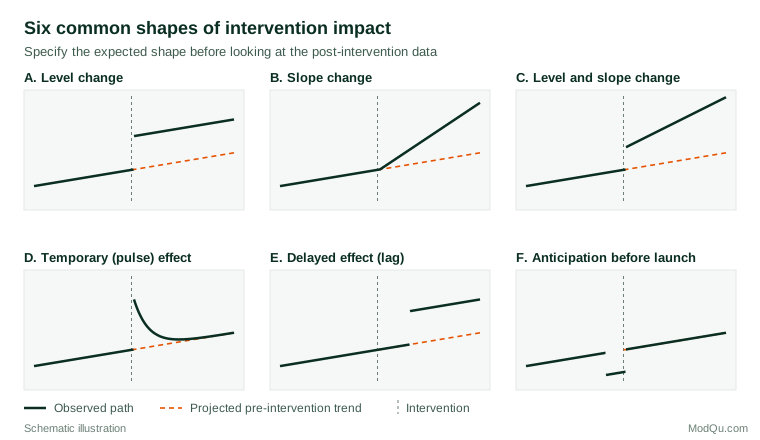
A flexible model fitted after seeing the data will almost always find some pattern, so the choice should rest on knowledge of how the intervention is supposed to work, with alternative shapes treated as sensitivity analyses rather than as a menu (Lopez Bernal et al., 2017).
Segmented regression
The workhorse analysis for ITS is segmented regression (Wagner et al., 2002). With time t measured in months from the start of the series, an indicator Xt equal to 1 from the intervention onwards and 0 before, and a counter of time since the intervention, the model for the outcome Yt is:
Yt = β0 + β1t + β2Xt + β3(t − T0)Xt + εt
Here T0 is the last pre-intervention period. The coefficients have direct interpretations:
- β0 is the baseline level at the start of the series.
- β1 is the pre-intervention trend per period.
- β2 is the immediate change in level when the intervention starts.
- β3 is the change in slope, the difference between the post- and pre-intervention trends.
The estimated effect at any point k periods after the intervention is β2 + β3k, the vertical gap between the fitted post-intervention line and the projected pre-intervention line. Reporting this gap at one or two meaningful horizons, such as six and twelve months, is usually clearer for decision-makers than reporting the coefficients alone (Penfold & Zhang, 2013).
For counts, such as weekly complaints, the same structure is used inside a Poisson or negative binomial regression, with an offset for the population at risk when it changes over time; effects are then expressed as rate ratios (Lopez Bernal et al., 2017). For proportions from surveys, a linear model on the percentage scale is often adequate when values stay well away from 0% and 100%, as in the example below.
A worked example: evaluating a sustainability campaign
Suppose a hypothetical consumer goods company runs a monthly tracker survey with 800 respondents per month. One question measures prompted awareness of the company's packaging-recycling programme. A national advertising campaign about the programme launched in month 25, and the tracker provides 24 months before and 12 months after. Figure 2 shows the illustrative data.
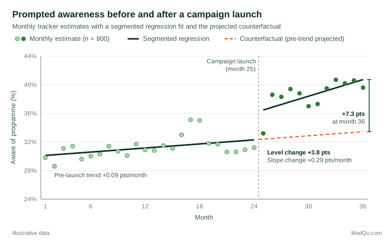
A naive comparison gives an average awareness of 31.2% before the launch and 38.6% after, a difference of 7.4 points. But awareness was already rising before the campaign, and the two periods are centred 18 months apart, so part of that difference would have happened anyway.
The segmented regression gives the following illustrative estimates, with 95% confidence intervals based on autocorrelation-robust standard errors:
| Term | Estimate | 95% CI |
|---|---|---|
| Pre-launch trend (β1) | +0.09 points per month | 0.00 to 0.19 |
| Level change at launch (β2) | +3.8 points | 1.6 to 6.0 |
| Slope change (β3) | +0.29 points per month | 0.03 to 0.56 |
The campaign is associated with an immediate rise of about 3.8 points and a steeper upward trend afterwards. By month 36 the fitted awareness is 40.7%, against a projected 33.4% without the campaign, an estimated effect of 7.3 points. The slope estimate, however, is imprecise: its interval runs from almost zero to more than half a point per month, so the claim that the effect is still growing is much weaker than the claim that there was an immediate rise. Twelve post-launch months is a short window in which to estimate a change in trend.
Autocorrelation and seasonality
Ordinary least squares assumes that the errors are independent. In time series, they rarely are: a month that is unusually high tends to be followed by another high month. In the example, the correlation between successive residuals is about 0.38 and the Durbin–Watson statistic is 1.23, well below the value of 2 expected under independence (Durbin & Watson, 1950). Positive autocorrelation makes ordinary standard errors too small and confidence intervals too narrow.
There are three common remedies. The first is to keep the ordinary estimates but use heteroskedasticity- and autocorrelation-consistent standard errors (Newey & West, 1987), as in the table above. The second is to model the error structure directly, for example with autoregressive errors, and check the residuals with a Ljung–Box test (Ljung & Box, 1978; Shumway & Stoffer, 2017). The third is the full intervention analysis of Box and Tiao (1975), which combines an ARIMA model for the noise with transfer functions for the intervention; it builds on the modelling approach of Box and Jenkins (1970) and was first illustrated with air pollution data from Los Angeles.
Seasonality is the other routine threat. Retail sales, travel bookings and many survey measures follow calendar patterns. If an intervention starts in a seasonally strong month, an unadjusted model will credit the season to the intervention. Seasonal indicator variables or Fourier terms can be added to the regression (Hyndman & Athanasopoulos, 2021), or the series can be seasonally adjusted first using a decomposition such as STL (Cleveland et al., 1990). Two full years of pre-intervention data make seasonality much easier to estimate.
Threats to validity
The main weakness of a single-series design is history: something else that happened at the same time as the intervention (Shadish et al., 2002). If a competitor withdrew from the market in month 25, or a news story about plastic waste ran that month, the campaign would receive credit for its effect. Other threats include:
- Instrumentation changes. A new survey supplier, a redesigned questionnaire or a change in mode at the intervention date can produce an apparent step.
- Selection and composition changes. If the population measured changes, for example because a loyalty programme attracts new customer types, the outcome can shift without any change in behaviour among existing customers.
- Regression to the mean. Interventions are often triggered by an unusually bad result. A long pre-intervention series helps show whether the starting point was atypical.
Several design additions strengthen the inference. A control series that was exposed to the same history but not to the intervention, such as a region where the campaign did not run or a brand that was not advertised, lets the analyst subtract shared shocks (Lopez Bernal et al., 2018). This combines ITS with the logic of difference-in-differences. When several untreated units are available, the synthetic control method builds a weighted combination of them that tracks the treated series before the intervention (Abadie et al., 2010). Brodersen et al. (2015) developed a related Bayesian structural time-series approach, designed for estimating the effect of marketing campaigns, that uses control series to predict the counterfactual.
Practical guidance for survey and business data
- Plan the evaluation before the launch. Agree the outcome, the intervention date, the expected shape of the effect and the comparison series in writing. This is the single most effective safeguard against post hoc storytelling.
- Hold the measurement constant. For tracker surveys, keep question wording, response scales, mode and sampling frame unchanged across the intervention. If a change is unavoidable, run the old and new versions in parallel for some months.
- Account for sampling error. Each survey wave is an estimate with its own margin of error. With small monthly samples, wave-to-wave noise can swamp moderate effects; pooling into quarters, or weighting each point by its precision, may help.
- Report the counterfactual. Show the projected pre-intervention trend on the chart, report the estimated gap at stated horizons, and give confidence intervals.
- Run sensitivity analyses. Vary the impact model, the length of the pre-period, the treatment of seasonality and the handling of a transition period, and report whether the conclusion survives.
Common mistakes
- Comparing averages instead of trends. A pre/post comparison of means ignores any existing trend and will often overstate or understate the effect.
- Ignoring autocorrelation. Ordinary least squares standard errors can be badly overconfident in time series.
- Choosing the impact model after seeing the data. A model that fits a jump at exactly the right month is not evidence that the intervention caused the jump.
- Extrapolating too far. The projected counterfactual becomes less credible the further it extends from the pre-intervention data, because a linear trend rarely continues indefinitely.
These problems are not hypothetical. Ramsay et al. (2003) reviewed interrupted time-series studies of behaviour change strategies in health care and found that many had been analysed inappropriately, for example by ignoring secular trends or autocorrelation, and that reanalysis sometimes changed the conclusions.
Key takeaways
An interrupted time-series design estimates the effect of an intervention by comparing what happened after it with a projection of the pre-intervention trend. It is often the strongest design available when a change applies to everyone at once and no randomised comparison is possible. Segmented regression provides interpretable estimates of the immediate change in level and the change in trend, and the gap between the fitted and projected lines gives the effect at any chosen horizon. Credible analyses need a well-defined intervention date, consistent measurement, enough time points, an impact model chosen in advance, and allowance for autocorrelation and seasonality. The design's main weakness is coincident events, and a control series is the best defence against them.
References
Abadie, A., Diamond, A., & Hainmueller, J. (2010). Synthetic control methods for comparative case studies: Estimating the effect of California's tobacco control program. Journal of the American Statistical Association, 105(490), 493–505. https://doi.org/10.1198/jasa.2009.ap08746
Box, G. E. P., & Jenkins, G. M. (1970). Time series analysis: Forecasting and control. Holden-Day.
Box, G. E. P., & Tiao, G. C. (1975). Intervention analysis with applications to economic and environmental problems. Journal of the American Statistical Association, 70(349), 70–79. https://doi.org/10.1080/01621459.1975.10480264
Brodersen, K. H., Gallusser, F., Koehler, J., Rémy, N., & Scott, S. L. (2015). Inferring causal impact using Bayesian structural time-series models. The Annals of Applied Statistics, 9(1), 247–274. https://doi.org/10.1214/14-AOAS788
Campbell, D. T. (1969). Reforms as experiments. American Psychologist, 24(4), 409–429. https://doi.org/10.1037/h0027982
Cleveland, R. B., Cleveland, W. S., McRae, J. E., & Terpenning, I. (1990). STL: A seasonal-trend decomposition procedure based on loess. Journal of Official Statistics, 6(1), 3–73.
Durbin, J., & Watson, G. S. (1950). Testing for serial correlation in least squares regression: I. Biometrika, 37(3–4), 409–428. https://doi.org/10.2307/2332391
Holland, P. W. (1986). Statistics and causal inference. Journal of the American Statistical Association, 81(396), 945–960. https://doi.org/10.1080/01621459.1986.10478354
Hyndman, R. J., & Athanasopoulos, G. (2021). Forecasting: Principles and practice (3rd ed.). OTexts.
Kohavi, R., Tang, D., & Xu, Y. (2020). Trustworthy online controlled experiments: A practical guide to A/B testing. Cambridge University Press. https://doi.org/10.1017/9781108653985
Kontopantelis, E., Doran, T., Springate, D. A., Buchan, I., & Reeves, D. (2015). Regression based quasi-experimental approach when randomisation is not an option: Interrupted time series analysis. BMJ, 350, Article h2750. https://doi.org/10.1136/bmj.h2750
Ljung, G. M., & Box, G. E. P. (1978). On a measure of lack of fit in time series models. Biometrika, 65(2), 297–303. https://doi.org/10.1093/biomet/65.2.297
Lopez Bernal, J., Cummins, S., & Gasparrini, A. (2017). Interrupted time series regression for the evaluation of public health interventions: A tutorial. International Journal of Epidemiology, 46(1), 348–355. https://doi.org/10.1093/ije/dyw098
Lopez Bernal, J., Cummins, S., & Gasparrini, A. (2018). The use of controls in interrupted time series studies of public health interventions. International Journal of Epidemiology, 47(6), 2082–2093. https://doi.org/10.1093/ije/dyy135
Newey, W. K., & West, K. D. (1987). A simple, positive semi-definite, heteroskedasticity and autocorrelation consistent covariance matrix. Econometrica, 55(3), 703–708. https://doi.org/10.2307/1913610
Penfold, R. B., & Zhang, F. (2013). Use of interrupted time series analysis in evaluating health care quality improvements. Academic Pediatrics, 13(6, Suppl.), S38–S44. https://doi.org/10.1016/j.acap.2013.08.002
Ramsay, C. R., Matowe, L., Grilli, R., Grimshaw, J. M., & Thomas, R. E. (2003). Interrupted time series designs in health technology assessment: Lessons from two systematic reviews of behavior change strategies. International Journal of Technology Assessment in Health Care, 19(4), 613–623. https://doi.org/10.1017/S0266462303000576
Shadish, W. R., Cook, T. D., & Campbell, D. T. (2002). Experimental and quasi-experimental designs for generalized causal inference. Houghton Mifflin.
Shumway, R. H., & Stoffer, D. S. (2017). Time series analysis and its applications: With R examples (4th ed.). Springer. https://doi.org/10.1007/978-3-319-52452-8
Wagner, A. K., Soumerai, S. B., Zhang, F., & Ross-Degnan, D. (2002). Segmented regression analysis of interrupted time series studies in medication use research. Journal of Clinical Pharmacy and Therapeutics, 27(4), 299–309. https://doi.org/10.1046/j.1365-2710.2002.00430.x
Zhang, F., Wagner, A. K., & Ross-Degnan, D. (2011). Simulation-based power calculation for designing interrupted time series analyses of health policy interventions. Journal of Clinical Epidemiology, 64(11), 1252–1261. https://doi.org/10.1016/j.jclinepi.2011.02.007