
Statistics · Causal inference
Instrumental Variables
How instrumental variables recover causal effects when hidden confounders bias ordinary regression, which assumptions they rest on, how to test instrument strength, and how to read the results.
Suppose a subscription business wants to know whether customers who install its mobile app go on to spend more. Comparing installers with non-installers is easy, but the comparison is almost certainly misleading. The customers who install an app are often the keenest, most engaged and most affluent, and they would probably have spent more anyway. Adding control variables helps only with the differences that were measured. Motivation, loyalty and household budget are rarely in the data set.
Instrumental variables (IV) offer a way out of this problem. An instrument is a variable that shifts the treatment of interest, here app installation, but has no other route to the outcome. If such a variable exists, the part of the variation in the treatment that it creates is "as good as random", and that part can be used to estimate a causal effect even when important confounders are unmeasured. The idea is one of the most influential in applied statistics and econometrics (Angrist & Krueger, 2001; Imbens, 2014) and is closely related to the analysis of randomised experiments in which not everyone does what they were assigned to do.
The problem instruments solve
Causal questions ask what would happen to an outcome if we changed a treatment. In the potential outcomes framework, each customer has one spending level if they install the app and another if they do not, and the causal effect is the difference between the two (Holland, 1986). We never see both for the same person, so we compare groups. That comparison is fair only if the groups are alike in everything else that affects the outcome.
When some common cause of the treatment and the outcome is unobserved, the treatment is called endogenous, and regression of the outcome on the treatment is biased. This is confounding in its most troublesome form, because no amount of adjustment for observed variables removes it. Reverse causation and measurement error in the treatment have similar effects.
Randomised experiments solve the problem by design: a coin toss decides the treatment. Instrumental variables borrow that logic, with the instrument playing the role of a coin toss that controls the treatment only partly.
A short history
The method was first set out in an appendix to Philip Wright's (1928) book on tariffs for animal and vegetable oils, where it was used to separate supply and demand curves from price and quantity data. Stock and Trebbi (2003) review the history and the long debate over whether Philip Wright or his son, the geneticist Sewall Wright, wrote the appendix. Sargan (1958) developed the general theory of estimation with several instruments. From the 1990s, economists used "natural experiments" as instruments, such as the quarter of the year in which a person was born, which affects how many years of schooling compulsory attendance laws require (Angrist & Krueger, 1991). Epidemiologists later adopted the approach, notably in Mendelian randomisation, in which genetic variants that are allocated at conception serve as instruments for modifiable exposures (Davey Smith & Ebrahim, 2003).
The three core assumptions
A variable Z is a valid instrument for the effect of a treatment D on an outcome Y if three conditions hold (Angrist et al., 1996; Hernán & Robins, 2006).
- Relevance. Z is associated with D. The instrument must actually move the treatment. This is the only assumption that can be checked directly in the data.
- Independence. Z is unrelated to the unmeasured confounders U, as if it had been randomly assigned. A genuinely randomised invitation meets this condition by design; a natural experiment has to be argued for.
- Exclusion restriction. Z affects Y only through D. There is no direct path from the instrument to the outcome, and no path through any other variable.
A directed acyclic graph makes these conditions easy to see (Pearl, 2009). Figure 1 shows the structure for the app example, in which the instrument is a randomly assigned email invitation to install the app.
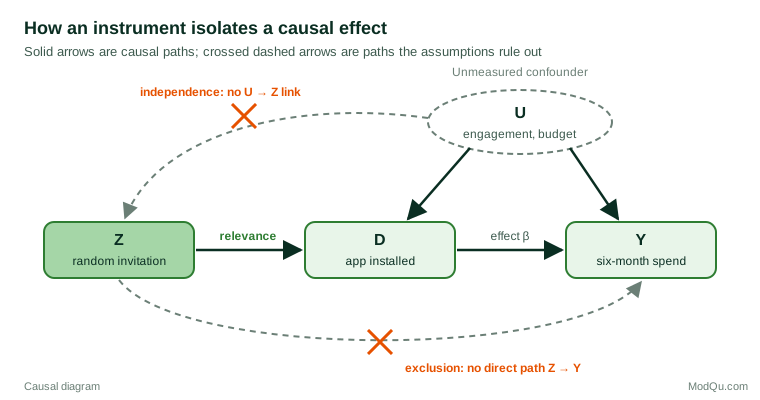
The exclusion restriction is usually the hardest assumption to defend. In the app example it would fail if the invitation email itself reminded customers to shop, raising spending whether or not they installed the app. It helps to list every other route from instrument to outcome and ask what evidence rules each one out.
Estimation
The Wald estimator
With a binary instrument and a binary treatment, the IV estimate is a simple ratio known as the Wald estimator. It divides the effect of the instrument on the outcome by the effect of the instrument on the treatment:
βIV = (E[Y | Z = 1] − E[Y | Z = 0]) ÷ (E[D | Z = 1] − E[D | Z = 0])
The numerator is the intention-to-treat (ITT) effect, or reduced form. The denominator is the first stage: how much the instrument changes the share of people treated. Because the instrument affects the outcome only through the treatment, scaling the ITT effect by the first stage gives the effect of the treatment itself. More generally, with one instrument and a continuous treatment, βIV = Cov(Z, Y) ÷ Cov(Z, D).
Two-stage least squares
When there are covariates or several instruments, the standard estimator is two-stage least squares (2SLS). In the first stage, the treatment is regressed on the instrument(s) and the covariates X:
D = π0 + π1Z + γX + v
In the second stage, the outcome is regressed on the fitted values of the treatment from the first stage, along with the same covariates:
Y = β0 + β1D̂ + δX + e
The coefficient β1 is the IV estimate. The fitted value D̂ contains only the variation in the treatment that the instrument produced, so it is free of the confounding that contaminates D itself. Running the two stages by hand gives the right estimate but wrong standard errors, so use software that fits 2SLS in one step (Angrist & Pischke, 2009).
A worked example
Consider a hypothetical retailer with 10,000 customers. It randomly emails half of them an invitation to install its new app. Six months later, the illustrative results are:
| Group | Customers | Share who installed the app | Mean six-month spend |
|---|---|---|---|
| Invited (Z = 1) | 5,000 | 40% | $520 |
| Not invited (Z = 0) | 5,000 | 10% | $502 |
The naive comparison is striking. In these illustrative data, customers who installed the app spent on average $601 and those who did not spent $481, a gap of $120. Much of that gap reflects who chooses to install, not what the app does.
The IV calculation uses only the random invitation. The ITT effect is $520 − $502 = $18 per invited customer. The first stage is 40% − 10% = 30 percentage points. The Wald estimate is therefore $18 ÷ 0.30 = $60. Installing the app raises six-month spending by about $60 for the customers whose installation decision was changed by the invitation, half the naive gap.
This example is an encouragement design: rather than forcing a treatment, the analyst randomises an encouragement to take it. The same logic applies to any randomised experiment with imperfect compliance, such as an online test in which some users assigned to a new feature never see it.
What the IV estimate means: compliers and the LATE
If the effect were the same for everyone, IV would estimate the population average effect. In practice effects vary. Imbens and Angrist (1994) and Angrist et al. (1996) showed that, under an additional assumption called monotonicity, IV estimates a local average treatment effect (LATE): the average effect among compliers, the people whose treatment status is changed by the instrument.
The framework sorts the population into four latent groups.
| Type | Treated if not encouraged? | Treated if encouraged? | Informative for IV? |
|---|---|---|---|
| Always-takers | Yes | Yes | No |
| Never-takers | No | No | No |
| Compliers | No | Yes | Yes |
| Defiers | Yes | No | Ruled out by monotonicity |
Monotonicity says there are no defiers: nobody is put off installing the app because they were invited. Always-takers and never-takers do the same thing whatever the instrument says, so they contribute nothing to the ITT effect. In the worked example, the 10% who installed without an invitation are always-takers, the 60% who did not install even when invited are never-takers, and the remaining 30% are compliers. The $60 estimate applies to that 30%.
The LATE is useful, but it is not always what a decision-maker wants. Compliers here are customers who respond to an email nudge; the effect for always-takers may be quite different. Different instruments define different complier groups, so two valid instruments can legitimately give different answers. Deaton (2010) stresses that this makes IV estimates hard to generalise beyond the setting in which the instrument operates. Imbens (2014) gives a balanced account of when the LATE answers a policy question and when it does not.
Weak instruments
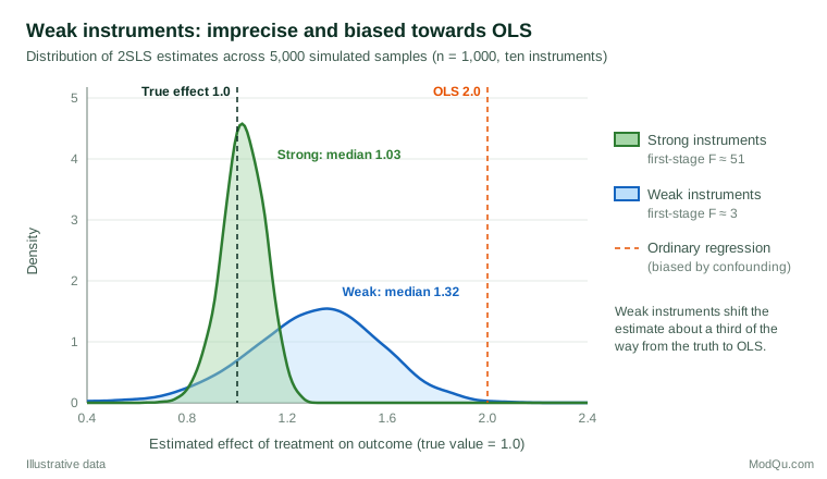
An instrument that only slightly moves the treatment is called weak. Weak instruments cause two serious problems. First, the IV estimate is very imprecise, because the first stage in the denominator is close to zero. Second, and less obviously, the estimate is biased towards the ordinary regression estimate it was meant to correct. In finite samples, the 2SLS bias is roughly 1/(F + 1) times the bias of ordinary least squares, where F is the first-stage F-statistic for the instruments (Angrist & Pischke, 2009). Conventional confidence intervals can also be far too narrow.
Bound et al. (1995) made the problem famous. They showed that the quarter-of-birth instruments used for the returns to schooling were weak in many specifications, and that randomly generated "instruments" with no real relationship to schooling produced results much like those obtained with the real ones. Figure 2 shows the same mechanism in a simulation.
How strong is strong enough?
Staiger and Stock (1997) proposed the widely used rule of thumb that the first-stage F-statistic should exceed 10. Stock et al. (2002) survey the problem and discuss critical values that link F to the maximum acceptable bias or test distortion, and Andrews et al. (2019) review the theory and practice in detail. More recent work argues that 10 is too lenient for ordinary t-tests: Lee et al. (2022) show that a conventional 5% test with one instrument needs a first-stage F above about 104.7 to have its stated size, and they provide adjusted critical values for weaker instruments.
The practical lessons are clear.
- Always report the first stage, including the coefficient on the instrument, its standard error and the F-statistic (using heteroscedasticity-robust or cluster-robust versions when appropriate).
- Use weak-instrument-robust inference when F is modest. The Anderson–Rubin test (Anderson & Rubin, 1949) remains valid however weak the instrument, and its confidence sets are a sound default (Andrews et al., 2019).
- Do not add many weak instruments to boost F. Using many instruments worsens the bias towards ordinary regression.
Testing what can be tested
Only relevance can be tested directly. The other assumptions can be probed, but never proved.
- Over-identification tests. With more instruments than treatments, the Sargan test (Sargan, 1958) and its robust variants ask whether the different instruments give consistent estimates. A rejection is a warning, but passing the test does not show that the instruments are valid: if all of them are biased in the same direction, the test has no power to detect it.
- Comparing IV and ordinary regression. The Hausman (1978) test asks whether the IV and ordinary regression estimates differ by more than chance. A large difference is evidence of endogeneity, provided the instrument is valid.
- Balance checks. Pre-instrument covariates should not differ across values of the instrument; imbalance casts doubt on independence.
- Falsification tests. An effect of the instrument in groups whose treatment it cannot change suggests the exclusion restriction fails.
Hernán and Robins (2006) warn that small violations of the exclusion or independence assumptions can produce large biases when the instrument is weak, because any direct effect of the instrument is divided by a small first stage. A weak and slightly invalid instrument can be worse than no instrument at all. Sensitivity analyses, in which the analyst asks how large a direct effect would have to be to change the conclusion, are a valuable complement to formal tests (Baiocchi et al., 2014).
Where instruments come from
Good instruments are rare, and most of the credibility of an IV study comes from the argument for the instrument rather than from the statistics (Angrist & Krueger, 2001). Common sources include the following.
- Randomised encouragement. Random invitations, reminders, discounts or default settings that change uptake of a product, service or programme. These are the strongest instruments available in business settings, because independence holds by design.
- Experiments with non-compliance. In a trial or online experiment where assignment is random but uptake is not, the random assignment is the instrument. Angrist et al. (1996) illustrate the approach with the Vietnam-era draft lottery as an instrument for military service.
- Natural experiments. Rules, thresholds, lotteries, weather, distance or timing that change exposure for reasons unrelated to the outcome. Each needs a careful case for exclusion.
- Provider or region preference. Differences between providers or areas in how often they use a treatment, although the assumptions are often contested (Baiocchi et al., 2014).
- Genetic variants. In Mendelian randomisation, variants associated with an exposure act as instruments (Davey Smith & Ebrahim, 2003), with the exclusion restriction threatened when one gene affects several traits.
Variables chosen because they happen to be in the data, such as demographics, are rarely convincing, because they usually affect outcomes directly.
Practical guidance for survey and business data
IV methods are well suited to several situations common in market and social research.
- Survey experiments with non-compliance. When respondents are randomly shown an advertisement, message or product sample but not all of them engage with it, the random assignment can instrument for actual exposure. The ITT effect answers "what happens if we show it"; the IV estimate answers "what happens to those who engage because we showed it". Both are worth reporting.
- Randomised incentives and reminders. Randomly varying an incentive or reminder can instrument for participation in a loyalty scheme, a webinar or a trial period, making it possible to estimate the effect of participation itself.
- Self-reported exposures. Survey measures of exposure are noisy, which biases ordinary regression towards zero; a valid instrument can correct this as well as confounding.
Some technical points matter in practice.
- Use the survey design. With weighted or clustered samples, fit 2SLS with survey weights and design-based or cluster-robust standard errors, and use robust versions of the first-stage F. When randomisation was by cluster, such as by store or region, inference must be at the cluster level.
- Plan for a large sample. IV estimates are much less precise than ordinary regression. Halving the first stage roughly doubles the standard error, so about four times the sample is needed for the same precision.
- Keep covariates pre-treatment. Adjusting for variables affected by the instrument or treatment can introduce new bias.
- Report the pieces. Show the first stage, the ITT effect and the IV estimate together, with the share of compliers. Readers can then judge whether a large IV estimate rests on a tiny first stage.
Common mistakes
- Treating IV as a cure for any endogeneity. IV replaces the untestable assumption of no unmeasured confounding with other untestable assumptions. It is only as credible as the instrument.
- Ignoring weak instruments. A first-stage F of 4 should change the conclusion, not just be noted in a footnote.
- Reading the LATE as a population effect. The estimate refers to compliers. Describe who they are, for example by comparing their observed characteristics with those of always-takers and never-takers, before generalising.
- Forgetting the exclusion restriction in encouragement designs. An encouragement can affect outcomes directly, for instance when an invitation email also advertises a sale.
- Not reporting transparently. Swanson and Hernán (2013) recommend that IV studies discuss each assumption explicitly and report enough detail for readers to judge them. Imbens and Rubin (2015) give a thorough treatment of these design questions.
How IV fits with other causal methods
Propensity score methods assume that all confounders are measured; difference-in-differences assumes parallel trends. A "fuzzy" regression discontinuity design, where crossing a threshold changes the probability of treatment, is analysed as an IV problem with the threshold as the instrument (Angrist & Pischke, 2009). Each design trades one set of assumptions for another, so agreement between designs is strong evidence.
Key takeaways
Instrumental variables estimate causal effects when hidden confounding would bias ordinary regression. The method depends on an instrument that moves the treatment, is as good as randomly assigned and affects the outcome only through the treatment. The estimate is the effect for compliers, the people whose behaviour the instrument changes. Weak instruments produce biased, overconfident results, so the first stage should always be reported and weak-instrument-robust inference used when it is modest. In business and survey research, the most credible instruments are usually randomised encouragements, and the best reports present the first stage, the intention-to-treat effect and the IV estimate side by side.
References
Anderson, T. W., & Rubin, H. (1949). Estimation of the parameters of a single equation in a complete system of stochastic equations. The Annals of Mathematical Statistics, 20(1), 46–63. https://doi.org/10.1214/aoms/1177730090
Andrews, I., Stock, J. H., & Sun, L. (2019). Weak instruments in instrumental variables regression: Theory and practice. Annual Review of Economics, 11, 727–753. https://doi.org/10.1146/annurev-economics-080218-025643
Angrist, J. D., Imbens, G. W., & Rubin, D. B. (1996). Identification of causal effects using instrumental variables. Journal of the American Statistical Association, 91(434), 444–455. https://doi.org/10.1080/01621459.1996.10476902
Angrist, J. D., & Krueger, A. B. (1991). Does compulsory school attendance affect schooling and earnings? The Quarterly Journal of Economics, 106(4), 979–1014. https://doi.org/10.2307/2937954
Angrist, J. D., & Krueger, A. B. (2001). Instrumental variables and the search for identification: From supply and demand to natural experiments. Journal of Economic Perspectives, 15(4), 69–85. https://doi.org/10.1257/jep.15.4.69
Angrist, J. D., & Pischke, J.-S. (2009). Mostly harmless econometrics: An empiricist's companion. Princeton University Press. https://doi.org/10.1515/9781400829828
Baiocchi, M., Cheng, J., & Small, D. S. (2014). Instrumental variable methods for causal inference. Statistics in Medicine, 33(13), 2297–2340. https://doi.org/10.1002/sim.6128
Bound, J., Jaeger, D. A., & Baker, R. M. (1995). Problems with instrumental variables estimation when the correlation between the instruments and the endogenous explanatory variable is weak. Journal of the American Statistical Association, 90(430), 443–450. https://doi.org/10.1080/01621459.1995.10476536
Davey Smith, G., & Ebrahim, S. (2003). 'Mendelian randomization': Can genetic epidemiology contribute to understanding environmental determinants of disease? International Journal of Epidemiology, 32(1), 1–22. https://doi.org/10.1093/ije/dyg070
Deaton, A. (2010). Instruments, randomization, and learning about development. Journal of Economic Literature, 48(2), 424–455. https://doi.org/10.1257/jel.48.2.424
Hausman, J. A. (1978). Specification tests in econometrics. Econometrica, 46(6), 1251–1271. https://doi.org/10.2307/1913827
Hernán, M. A., & Robins, J. M. (2006). Instruments for causal inference: An epidemiologist's dream? Epidemiology, 17(4), 360–372. https://doi.org/10.1097/01.ede.0000222409.00878.37
Holland, P. W. (1986). Statistics and causal inference. Journal of the American Statistical Association, 81(396), 945–960. https://doi.org/10.1080/01621459.1986.10478354
Imbens, G. W. (2014). Instrumental variables: An econometrician's perspective. Statistical Science, 29(3), 323–358. https://doi.org/10.1214/14-STS480
Imbens, G. W., & Angrist, J. D. (1994). Identification and estimation of local average treatment effects. Econometrica, 62(2), 467–475. https://doi.org/10.2307/2951620
Imbens, G. W., & Rubin, D. B. (2015). Causal inference for statistics, social, and biomedical sciences: An introduction. Cambridge University Press. https://doi.org/10.1017/CBO9781139025751
Lee, D. S., McCrary, J., Moreira, M. J., & Porter, J. (2022). Valid t-ratio inference for IV. American Economic Review, 112(10), 3260–3290. https://doi.org/10.1257/aer.20211063
Pearl, J. (2009). Causality: Models, reasoning, and inference (2nd ed.). Cambridge University Press. https://doi.org/10.1017/CBO9780511803161
Sargan, J. D. (1958). The estimation of economic relationships using instrumental variables. Econometrica, 26(3), 393–415. https://doi.org/10.2307/1907619
Staiger, D., & Stock, J. H. (1997). Instrumental variables regression with weak instruments. Econometrica, 65(3), 557–586. https://doi.org/10.2307/2171753
Stock, J. H., & Trebbi, F. (2003). Retrospectives: Who invented instrumental variable regression? Journal of Economic Perspectives, 17(3), 177–194. https://doi.org/10.1257/089533003769204416
Stock, J. H., Wright, J. H., & Yogo, M. (2002). A survey of weak instruments and weak identification in generalized method of moments. Journal of Business & Economic Statistics, 20(4), 518–529. https://doi.org/10.1198/073500102288618658
Swanson, S. A., & Hernán, M. A. (2013). Commentary: How to report instrumental variable analyses (suggestions welcome). Epidemiology, 24(3), 370–374. https://doi.org/10.1097/EDE.0b013e31828d0590
Wright, P. G. (1928). The tariff on animal and vegetable oils. Macmillan.