
Statistics · Causal inference
Propensity Score Matching
How propensity score matching builds comparable groups from observational data, how to check that it worked, and why it cannot fix confounders that were never measured.
Businesses constantly want to know whether something they did made a difference. Did joining the loyalty programme make customers spend more? Did attending the product webinar raise purchase intent? Did the premium support tier reduce churn? A randomised controlled trial answers such questions cleanly, but most of the time the data come from people who chose for themselves. Loyalty members differ from non-members before they ever join: they tend to shop more, earn more and engage more. Comparing the two groups directly mixes the effect of the programme with the effect of who signs up.
Propensity score matching is one of the most widely used ways to reduce this problem in observational data. It pairs each treated person with one or more untreated people who had a similar chance of being treated, given what was measured about them, and then compares outcomes within the matched sample. The idea was set out by Rosenbaum and Rubin (1983) and has since become a standard tool in medicine, economics, public policy and marketing analytics (Stuart, 2010).
The problem matching tries to solve
Causal questions are easiest to state in terms of potential outcomes (Rubin, 1974; Holland, 1986). Each customer has two possible spending levels: one if they join the programme and one if they do not. Only one is ever observed. The unobserved one is the counterfactual, and the causal effect for that customer is the difference between the two.
Because we never see both outcomes for the same person, we compare groups instead. Randomisation makes groups comparable on average in every respect, measured or not. Without randomisation, the members and non-members differ systematically, and the raw difference in their outcomes contains selection bias. When the variables that drive both joining and spending also differ between the groups, the comparison suffers from confounding.
The classic remedy is to compare like with like: members aged 35 to 44 with high prior spend against non-members aged 35 to 44 with high prior spend, and so on. With more than a few covariates, though, exact matching quickly runs out of people, because almost nobody shares the same values on ten variables at once.
What the propensity score is
The propensity score is the probability that a person receives the treatment given their observed covariates:
e(x) = P(T = 1 | X = x)
Rosenbaum and Rubin (1983) proved two results that make this single number so useful. First, it is a balancing score: among people with the same propensity score, the distribution of the observed covariates is the same in the treated and untreated groups. Second, if treatment assignment is "strongly ignorable" given the covariates, it is also ignorable given the propensity score alone. Strong ignorability has two parts:
- No unmeasured confounding. Given the observed covariates, treatment is unrelated to the potential outcomes. Everything that affects both joining and spending has been measured.
- Overlap (common support). Every type of person has some chance of being treated and some chance of not being treated: 0 < e(x) < 1.
Under these conditions, matching on one number achieves what exact matching on many covariates would achieve, which turns a high-dimensional problem into a one-dimensional one.
How propensity score matching works
In practice the method follows a sequence of design steps, ideally completed before anyone looks at the outcome data (Rubin, 2007; Stuart, 2010).
- Choose the covariates. Include variables that influence both treatment and outcome, measured before treatment. Do not include variables that could themselves be affected by the treatment, such as satisfaction measured after joining.
- Estimate the propensity score. Logistic regression of treatment on the covariates is the usual choice, though flexible models such as boosted trees are also used. The aim is balance, not prediction, so a model that predicts treatment extremely well is not necessarily better.
- Match. The simplest algorithm is 1:1 nearest-neighbour matching: each treated unit is paired with the untreated unit whose score is closest. A caliper sets a maximum allowed distance; a commonly used caliper is 0.2 standard deviations of the logit of the propensity score (Austin, 2011). Other options include matching with replacement, matching several controls per treated unit, and optimal matching (Rosenbaum & Rubin, 1985; Caliendo & Kopeinig, 2008).
- Check balance. Compare the covariate distributions of the matched groups. If balance is poor, revise the propensity model or the matching method and repeat.
- Estimate the effect. Compare outcomes in the matched sample, usually as a difference in means or proportions, often with a regression adjustment for any remaining imbalance.
Ho et al. (2007) describe this approach as preprocessing: matching first, then fitting a model to the matched data, makes the final estimate much less sensitive to the exact form of that model. Heckman et al. (1997) showed that matching performs best when treated and comparison groups come from the same local markets and are measured with the same questionnaire, a point that applies directly to survey data.
Checking balance
Balance is assessed on the covariates, not on p-values. The standard diagnostic is the standardised mean difference for each covariate:
d = (x̄T − x̄C) ÷ √[(sT2 + sC2) ÷ 2]
Here x̄ and s are the mean and standard deviation in the treated (T) and comparison (C) groups. An absolute value below 0.1 is widely treated as negligible imbalance. Austin (2009) recommends standardised differences and graphical checks over significance tests, because significance tests depend on sample size and the matched sample is smaller than the original one. Variance ratios and plots of the full distributions add useful detail.
A worked example
Consider a hypothetical retailer that surveys 4,200 customers and links the responses to purchase records. Of these, 900 joined the loyalty programme last year. Members spent an average of $1,480 in the following year and non-members $960, a raw difference of $520. Few analysts would credit the programme with all of it: members were already heavier shoppers.
The analyst estimates a propensity score from seven pre-enrolment covariates using logistic regression, then performs 1:1 nearest-neighbour matching with a caliper of 0.2 standard deviations of the logit. Forty members with very high scores have no suitable match and are dropped, leaving 860 matched pairs. Figure 1 shows the balance before and after matching.
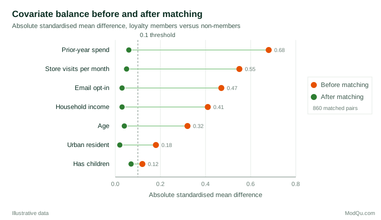
Before matching, all seven covariates exceed the 0.1 threshold, with prior-year spend the most unbalanced. After matching, all differences are 0.07 or less. In the matched sample, members spent $1,410 and their matched non-members $1,220, an estimated effect of $190 per member (hypothetical 95% confidence interval $120 to $260). Most of the raw $520 gap reflected who joins rather than what the programme did. For a business case, that difference is decisive: a programme judged on the raw gap would look nearly three times as profitable as the matched analysis suggests, and budgets set on that basis would be badly overstated.
Two features of this estimate matter for interpretation. It is the average treatment effect on the treated (ATT): the effect for customers like those who joined, not for all customers. Imbens (2004) explains why this target and the average effect across the whole population can differ substantially. It also excludes the 40 members without matches, so it describes the region of common support only.
Uncertainty and inference
Standard errors for matching estimators need care. The matched pairs are not independent draws, and the matching itself is estimated from the data. Abadie and Imbens (2006) derived the large-sample properties of nearest-neighbour matching estimators, showing that they carry a bias term when matching on several continuous covariates and proposing variance estimators and bias corrections. In practice, analysts often use cluster-robust standard errors with the matched pair or set as the cluster, or software that implements these corrections.
Alternatives that use the same score
Matching is only one way to use the propensity score. Others include:
- Subclassification, which groups units into strata, often five, by propensity score and averages the within-stratum differences (Rosenbaum & Rubin, 1983).
- Inverse probability of treatment weighting, which weights each person by the inverse of the probability of the treatment they actually received. It keeps the whole sample but can be unstable when some scores are close to 0 or 1. Austin and Stuart (2015) give practical guidance on diagnostics and reporting.
- Covariate adjustment, which includes the score in an outcome regression.
Each answers a slightly different question and has different weaknesses. Austin (2011) gives an accessible comparison, and Imbens and Rubin (2015) treat the subject in depth.
Practical guidance for survey and business data
- Measure confounders before treatment. In a cross-sectional survey, many covariates are measured after the treatment and may have been changed by it. Purchase records, sign-up dates and earlier waves of a tracker help establish the time order.
- Use the survey weights. When the sample comes from a complex or weighted design, the matched estimate describes the sample unless weights are carried through. DuGoff et al. (2014) recommend including the survey weight as a covariate in the propensity model and using the weights in the outcome analysis when the aim is to generalise to the population.
- Report what was dropped. Units outside common support change the population to which the estimate applies. State how many were excluded and how they differ.
- Keep the outcome out of the design stage. Choosing the matching method because it gives the "right" answer invalidates the inference (Rubin, 2007).
- Benchmark where possible. Dehejia and Wahba (1999) showed that propensity score methods reproduced an experimental estimate for a job-training programme reasonably well when the covariates were rich, but the same literature also shows how sensitive results can be to the choice of comparison group.
Limitations and common mistakes
The most important limitation is that matching can only balance what has been measured. If customers who join the loyalty programme are also more brand-loyal in ways the survey did not capture, the matched estimate will still be biased, however good the balance plot looks. Rosenbaum (2002) developed sensitivity analyses that ask how strong an unmeasured confounder would have to be to change the conclusion. VanderWeele and Ding (2017) proposed the E-value, the minimum strength of association an unmeasured confounder would need with both treatment and outcome to explain away an observed effect.
Other common mistakes include:
- Treating propensity score matching as a guarantee. King and Nielsen (2019) show that matching on the propensity score, and especially pruning more observations after balance is already good, can increase imbalance and model dependence. They recommend checking balance directly and considering alternatives such as Mahalanobis distance matching.
- Conditioning on post-treatment variables, which can introduce bias rather than remove it.
- Testing balance with p-values instead of standardised differences (Austin, 2009).
- Ignoring poor overlap. When the treated and untreated groups barely overlap in their scores, no method can produce a credible comparison for the units outside the shared range.
Key takeaways
Propensity score matching turns many covariates into a single score and builds a comparison group that resembles the treated group on everything that was measured. Done well, it separates the design of an observational study from its analysis, makes the comparison transparent and reduces dependence on modelling choices. Its credibility rests on two assumptions: that all important confounders were measured before treatment, and that the groups overlap. Check balance with standardised differences, report the estimand and the units dropped, use survey weights where needed and pair the estimate with a sensitivity analysis for unmeasured confounding.
References
Abadie, A., & Imbens, G. W. (2006). Large sample properties of matching estimators for average treatment effects. Econometrica, 74(1), 235–267. https://doi.org/10.1111/j.1468-0262.2006.00655.x
Austin, P. C. (2009). Balance diagnostics for comparing the distribution of baseline covariates between treatment groups in propensity-score matched samples. Statistics in Medicine, 28(25), 3083–3107. https://doi.org/10.1002/sim.3697
Austin, P. C. (2011). An introduction to propensity score methods for reducing the effects of confounding in observational studies. Multivariate Behavioral Research, 46(3), 399–424. https://doi.org/10.1080/00273171.2011.568786
Austin, P. C., & Stuart, E. A. (2015). Moving towards best practice when using inverse probability of treatment weighting (IPTW) using the propensity score to estimate causal treatment effects in observational studies. Statistics in Medicine, 34(28), 3661–3679. https://doi.org/10.1002/sim.6607
Caliendo, M., & Kopeinig, S. (2008). Some practical guidance for the implementation of propensity score matching. Journal of Economic Surveys, 22(1), 31–72. https://doi.org/10.1111/j.1467-6419.2007.00527.x
Dehejia, R. H., & Wahba, S. (1999). Causal effects in nonexperimental studies: Reevaluating the evaluation of training programs. Journal of the American Statistical Association, 94(448), 1053–1062. https://doi.org/10.1080/01621459.1999.10473858
DuGoff, E. H., Schuler, M., & Stuart, E. A. (2014). Generalizing observational study results: Applying propensity score methods to complex surveys. Health Services Research, 49(1), 284–303. https://doi.org/10.1111/1475-6773.12090
Heckman, J. J., Ichimura, H., & Todd, P. E. (1997). Matching as an econometric evaluation estimator: Evidence from evaluating a job training programme. The Review of Economic Studies, 64(4), 605–654. https://doi.org/10.2307/2971733
Ho, D. E., Imai, K., King, G., & Stuart, E. A. (2007). Matching as nonparametric preprocessing for reducing model dependence in parametric causal inference. Political Analysis, 15(3), 199–236. https://doi.org/10.1093/pan/mpl013
Holland, P. W. (1986). Statistics and causal inference. Journal of the American Statistical Association, 81(396), 945–960. https://doi.org/10.1080/01621459.1986.10478354
Imbens, G. W. (2004). Nonparametric estimation of average treatment effects under exogeneity: A review. The Review of Economics and Statistics, 86(1), 4–29. https://doi.org/10.1162/003465304323023651
Imbens, G. W., & Rubin, D. B. (2015). Causal inference for statistics, social, and biomedical sciences: An introduction. Cambridge University Press. https://doi.org/10.1017/CBO9781139025751
King, G., & Nielsen, R. (2019). Why propensity scores should not be used for matching. Political Analysis, 27(4), 435–454. https://doi.org/10.1017/pan.2019.11
Rosenbaum, P. R. (2002). Observational studies (2nd ed.). Springer. https://doi.org/10.1007/978-1-4757-3692-2
Rosenbaum, P. R., & Rubin, D. B. (1983). The central role of the propensity score in observational studies for causal effects. Biometrika, 70(1), 41–55. https://doi.org/10.1093/biomet/70.1.41
Rosenbaum, P. R., & Rubin, D. B. (1985). Constructing a control group using multivariate matched sampling methods that incorporate the propensity score. The American Statistician, 39(1), 33–38. https://doi.org/10.1080/00031305.1985.10479383
Rubin, D. B. (1974). Estimating causal effects of treatments in randomized and nonrandomized studies. Journal of Educational Psychology, 66(5), 688–701. https://doi.org/10.1037/h0037350
Rubin, D. B. (2007). The design versus the analysis of observational studies for causal effects: Parallels with the design of randomized trials. Statistics in Medicine, 26(1), 20–36. https://doi.org/10.1002/sim.2739
Stuart, E. A. (2010). Matching methods for causal inference: A review and a look forward. Statistical Science, 25(1), 1–21. https://doi.org/10.1214/09-STS313
VanderWeele, T. J., & Ding, P. (2017). Sensitivity analysis in observational research: Introducing the E-value. Annals of Internal Medicine, 167(4), 268–274. https://doi.org/10.7326/M16-2607