
Statistics · Causal inference
Synthetic Control Methods for Comparative Case Knowledge
How the synthetic control method builds a weighted comparison unit to estimate the effect of an intervention on a single region, market or organisation, and how to judge whether the result is credible.
Some of the most important business questions concern a single case. A retailer rolls out a new store format in one province. A regulator changes the rules in one market. A brand runs a heavy advertising campaign in one region before deciding whether to go national. There is only one treated unit, so there is no sample of treated cases to average over, and the untreated regions all differ from the treated one in obvious ways. Simple before-and-after comparisons confuse the intervention with everything else that changed at the same time.
The synthetic control method offers a disciplined answer. Instead of choosing one comparison region by judgement, it builds a weighted average of several untreated units that together reproduce the treated unit's history as closely as possible. The weighted average, the synthetic control, then stands in for what would have happened without the intervention. The method was introduced by Abadie and Gardeazabal (2003) and developed by Abadie et al. (2010, 2015). Athey and Imbens (2017) described it as arguably the most important innovation in the policy evaluation literature of the previous fifteen years.
The comparative case study problem
In the language of potential outcomes, each region has an outcome it would show with the intervention and an outcome it would show without it (Rubin, 1974). After the intervention, we observe only the first for the treated region. The second is the counterfactual, and estimating it is the whole problem.
Comparative case studies have long tackled this by finding a similar place: a neighbouring region, a comparable country, a sister brand. The weakness is that the choice is subjective and its quality hard to judge. Difference-in-differences, the standard quantitative alternative, compares the change in the treated unit with the change in a control group and assumes that, without the intervention, both would have moved in parallel (Angrist & Pischke, 2009). When the treated unit has followed a different trajectory from the average control, that assumption fails. Difference-in-differences studies with many periods also tend to understate their uncertainty when outcomes are correlated over time (Bertrand et al., 2004).
The synthetic control method replaces the analyst's choice of comparison with a transparent, data-driven one, and makes it easy to see whether the comparison is any good.
How a synthetic control is built
Suppose there is one treated unit, labelled 1, and J untreated units in a donor pool, observed over periods t = 1, …, T. The intervention starts after period T0. A synthetic control is a set of weights w2, …, wJ+1, one for each donor, that are non-negative and sum to one. The estimated counterfactual and the estimated effect in each post-intervention period are:
Ŷ1t(0) = Σj wj Yjt and τ̂t = Y1t − Σj wj Yjt
The weights are chosen so that the synthetic control matches the treated unit as closely as possible before the intervention, on the pre-intervention outcomes and on predictors of the outcome such as population, income or market size (Abadie et al., 2010). Software for the original method weights the predictors by their importance in predicting the outcome (Abadie et al., 2011).
Three features of this construction matter in practice:
- No extrapolation. Because the weights are non-negative and sum to one, the synthetic control is an interpolation among real units. It cannot invent a region more extreme than any in the donor pool (Abadie, 2021).
- Sparsity and transparency. The solution usually gives positive weight to only a few donors. Readers can see exactly which units form the comparison and in what proportions, and judge whether that makes substantive sense.
- Design before outcomes. The weights are fixed using only pre-intervention data. They can be computed, and their fit inspected, before anyone looks at post-intervention results, which limits the scope for tuning the analysis to get a desired answer.
Why should matching the past predict the future? Abadie et al. (2010) showed that if outcomes are driven by a set of unobserved common factors, each affecting units to a different degree, then a synthetic control that tracks the treated unit closely over a long pre-intervention period must also approximately match its exposure to those factors. This is a weaker requirement than the parallel trends assumption of difference-in-differences, which in effect gives every control unit the same weight.
Classic applications
The first application estimated the economic cost of terrorism in the Basque Country, comparing its per capita GDP with that of a synthetic Basque Country built from other Spanish regions (Abadie & Gardeazabal, 2003). The best-known application examined California's Proposition 99, a tobacco control programme passed in 1988. Using a synthetic California made from other US states, Abadie et al. (2010) estimated that by 2000 annual per capita cigarette sales in California were about 26 packs lower than they would have been without the programme. Abadie et al. (2015) applied the method to the economic effect of German reunification on West Germany, using a synthetic West Germany constructed from other industrialised countries.
Applications have since spread to health policy (Kreif et al., 2016; Bouttell et al., 2018), economic development and disasters (Cavallo et al., 2013) and marketing, where the intervention is often a regional campaign or launch.
A worked example
Consider a hypothetical brand that tracks consideration, the percentage of category buyers who would consider buying it, through a monthly survey in 16 sales regions. In month 25 the brand launches an intensive regional campaign in Region A only. The question is how much the campaign raised consideration in Region A over the following 12 months.
A simple before-and-after comparison is misleading. In the illustrative data, consideration in Region A averaged 41.2% before the campaign and 42.4% after it, a rise of about 1.3 points. But consideration was drifting downwards across the category in the second year, so the before-and-after comparison understates the campaign's contribution.
The synthetic control is built from the other 15 regions, using the 24 pre-campaign months. The optimisation gives positive weight to seven regions, with most of the weight on four of them:
| Donor region | Weight |
|---|---|
| Region K | 0.22 |
| Region N | 0.21 |
| Region G | 0.19 |
| Region P | 0.17 |
| Region I | 0.08 |
| Region D | 0.07 |
| Region L | 0.06 |
| Other eight regions | 0.00 |
Figure 1 shows the result. Before the campaign, the synthetic Region A tracks the real one closely, including its seasonal pattern; the root mean squared prediction error (RMSPE) over the 24 months is 0.37 points. After the campaign, the two lines separate. The real Region A averages 42.4% while its synthetic counterpart averages 39.4%, an estimated average effect of about 3.0 points, rising to about 3.5 points in the last six months.
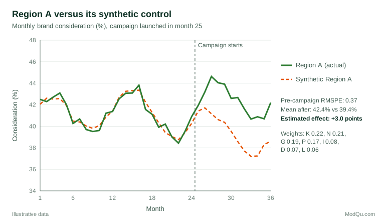
A difference-in-differences comparison against the simple average of all 15 other regions gives about 2.9 points in this example, close to the synthetic control estimate. That agreement is reassuring rather than guaranteed: when the treated unit differs more from the average donor, the two methods can diverge sharply, and the synthetic control's pre-period fit shows which comparison deserves more trust.
Inference with placebo tests
With one treated unit, conventional standard errors are not available: there is no sample of treated units to compute them from. The original papers proposed inference by placebo tests, which ask how unusual the estimated effect is compared with effects estimated where no intervention happened (Abadie et al., 2010, 2015).
In an in-space placebo test, the method is applied to each donor region in turn as if it had been treated, using the remaining regions as its donor pool. If the estimated gap for Region A is large relative to the placebo gaps, the result is unlikely to be an artefact of the method. Because some placebo units are fitted poorly before the intervention, a common summary is the ratio of post-intervention to pre-intervention RMSPE, which scales each unit's post-period gap by how well it was fitted beforehand.
Figure 2 shows the gaps for Region A and the 15 placebo regions, each fitted without Region A in its donor pool so that the campaign cannot leak into the placebo comparisons. Most placebo gaps stay within about 2 points of zero. Two are more striking. Region K, whose history is unusual and hard to reproduce from the others, was fitted poorly before month 25 (pre-period RMSPE 1.17, about three times Region A's) and drifts upwards afterwards, briefly reaching about 4 points. Region N drifts about 2 points below zero. Looking at raw gaps alone, Region K might seem to rival Region A. Scaling by pre-period fit resolves this: Region A's ratio is about 8.6, while the largest placebo ratio, Region N's, is about 2.5 and Region K's is about 2.2. Region A ranks first of 16, so the permutation p-value is 1/16, or about 0.06. This illustrates an important limit: with 16 units, 0.0625 is the smallest p-value the test can produce, however large the effect. Some analysts also drop placebo units whose pre-period fit is much worse than the treated unit's before comparing gaps (Abadie et al., 2010).
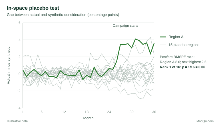
Two further checks are standard. An in-time placebo moves the intervention date back to a period when nothing happened; a credible method should find no effect there. A leave-one-out analysis drops each heavily weighted donor in turn to show that the result does not depend on one region (Abadie et al., 2015; Abadie, 2021).
Formal inference has since developed further. Firpo and Possebom (2018) set out the permutation test more formally and added sensitivity analysis and confidence sets. Chernozhukov et al. (2021) proposed conformal inference methods that permute residuals over time and provide exact or approximately valid tests under stated conditions.
When the method is credible
Abadie (2021) sets out the conditions under which synthetic controls are most convincing. Several apply directly to business data:
- A long pre-intervention period. A close fit over many periods, including seasonal cycles, is far more persuasive than a fit over a few points, which may simply reflect overfitting to noise.
- Good pre-intervention fit. If no combination of donors can reproduce the treated unit's history, the synthetic control is not a credible counterfactual. Ferman and Pinto (2021) showed that with imperfect pre-intervention fit the estimator can be biased, and suggested modifications, such as allowing for differences in levels, that reduce the problem.
- A suitable donor pool. Donors should be similar in kind to the treated unit and unaffected by the intervention. Regions that receive spillover advertising, or competitors that react to a launch, should be excluded.
- No anticipation and no coincident shocks. If customers change behaviour in expectation of the intervention, or if something else happens only in the treated unit at the same time, the gap will capture that too.
- Effect size relative to volatility. Effects small relative to the normal month-to-month noise of the outcome are hard to detect with any method.
Extensions and alternatives
The basic method has been extended in several directions, mostly to deal with imperfect fit, many treated units or staggered timing:
- Augmented synthetic control adds an outcome model, such as ridge regression, to correct the bias that remains when the pre-intervention fit is imperfect (Ben-Michael et al., 2021).
- Synthetic difference-in-differences combines synthetic control unit weights with time weights and the fixed effects of difference-in-differences, and performs well across a range of settings (Arkhangelsky et al., 2021).
- The generalised synthetic control method estimates an interactive fixed effects model and handles several treated units with different start dates (Xu, 2017).
- Matrix completion treats the missing untreated outcomes as missing entries in a matrix of units by periods, and includes synthetic control and unconfoundedness approaches as special cases (Athey et al., 2021).
- Penalised synthetic control trades off aggregate fit against the distance between the treated unit and each donor, which gives a unique solution when many treated units are studied with disaggregated data (Abadie & L'Hour, 2021).
- Regression-based panel approaches use the donors' outcomes as regressors without the weight constraints (Hsiao et al., 2012), and Bayesian structural time-series models produce a counterfactual forecast with a full posterior distribution, an approach widely used for marketing interventions (Brodersen et al., 2015).
These methods relax the constraints of the original estimator in exchange for more modelling assumptions. In practice, reporting the basic synthetic control alongside one or two of these alternatives shows whether the conclusion depends on the method.
Practical guidance for survey and business data
- Account for sampling error in survey outcomes. When the outcome comes from a survey, each regional monthly estimate carries sampling error. A month with a few hundred interviews can move by several points by chance alone. Larger regional samples, rolling averages or modelled estimates reduce the noise, but the placebo test should be run on the same smoothed series as the main analysis.
- Fix the design before the outcome. Decide the donor pool, predictors, pre-period and outcome definition before looking at post-intervention data. Ferman et al. (2020) showed that trying many specifications gives analysts room to select a favourable result, and recommend reporting results across specifications.
- Plan campaigns with evaluation in mind. If a test region is chosen for convenience, it may be atypical of every other region. Choosing a test region that lies within the range of the donor pool, and keeping several comparable regions free of the intervention, makes a credible synthetic control possible.
- Watch for spillovers. National media, online advertising and travelling customers can carry a regional campaign into donor regions, biasing the estimate towards zero.
- Report the weights and the fit. Show the donor weights, the pre-period fit, the placebo distribution and the leave-one-out results, not just the headline effect.
- Translate the effect into business terms, with its uncertainty. A gain of 3 consideration points in one region is easier to act on when it is expressed as additional buyers or revenue and compared with the campaign's cost. Present the placebo range alongside it, so that decision-makers see how large an effect would have to be before it stood out from ordinary regional variation, and avoid presenting a single-region estimate as a forecast for a national roll-out.
Common mistakes
- Interpreting a poor fit as an effect. If the synthetic control never matched the treated unit, a post-intervention gap tells us nothing.
- Including affected units in the donor pool. Donors that received some of the treatment, or reacted to it, contaminate the counterfactual.
- Over-reading a p-value from a small donor pool. With 10 donors the smallest possible permutation p-value is 1/11, about 0.09.
- Matching on too few periods. A handful of pre-period points can be matched by many weight combinations, most of them meaningless.
- Ignoring other events. A synthetic control estimates the combined effect of everything that happened only to the treated unit after the start date.
Key takeaways
The synthetic control method estimates the effect of an intervention on a single unit by building a weighted combination of untreated units that reproduces the treated unit's past. Its strengths are transparency, the absence of extrapolation and a built-in visual test of credibility. Its results deserve confidence only when the pre-intervention fit is close over a long period, the donor pool is clean and placebo tests show the effect to be unusual. Used with care, it brings quantitative discipline to the comparative case studies that business decisions so often rely on.
References
Abadie, A. (2021). Using synthetic controls: Feasibility, data requirements, and methodological aspects. Journal of Economic Literature, 59(2), 391–425. https://doi.org/10.1257/jel.20191450
Abadie, A., Diamond, A., & Hainmueller, J. (2010). Synthetic control methods for comparative case studies: Estimating the effect of California's tobacco control program. Journal of the American Statistical Association, 105(490), 493–505. https://doi.org/10.1198/jasa.2009.ap08746
Abadie, A., Diamond, A., & Hainmueller, J. (2011). Synth: An R package for synthetic control methods in comparative case studies. Journal of Statistical Software, 42(13), 1–17. https://doi.org/10.18637/jss.v042.i13
Abadie, A., Diamond, A., & Hainmueller, J. (2015). Comparative politics and the synthetic control method. American Journal of Political Science, 59(2), 495–510. https://doi.org/10.1111/ajps.12116
Abadie, A., & Gardeazabal, J. (2003). The economic costs of conflict: A case study of the Basque Country. American Economic Review, 93(1), 113–132. https://doi.org/10.1257/000282803321455188
Abadie, A., & L'Hour, J. (2021). A penalized synthetic control estimator for disaggregated data. Journal of the American Statistical Association, 116(536), 1817–1834. https://doi.org/10.1080/01621459.2021.1971535
Angrist, J. D., & Pischke, J.-S. (2009). Mostly harmless econometrics: An empiricist's companion. Princeton University Press. https://doi.org/10.1515/9781400829828
Arkhangelsky, D., Athey, S., Hirshberg, D. A., Imbens, G. W., & Wager, S. (2021). Synthetic difference-in-differences. American Economic Review, 111(12), 4088–4118. https://doi.org/10.1257/aer.20190159
Athey, S., Bayati, M., Doudchenko, N., Imbens, G., & Khosravi, K. (2021). Matrix completion methods for causal panel data models. Journal of the American Statistical Association, 116(536), 1716–1730. https://doi.org/10.1080/01621459.2021.1891924
Athey, S., & Imbens, G. W. (2017). The state of applied econometrics: Causality and policy evaluation. Journal of Economic Perspectives, 31(2), 3–32. https://doi.org/10.1257/jep.31.2.3
Ben-Michael, E., Feller, A., & Rothstein, J. (2021). The augmented synthetic control method. Journal of the American Statistical Association, 116(536), 1789–1803. https://doi.org/10.1080/01621459.2021.1929245
Bertrand, M., Duflo, E., & Mullainathan, S. (2004). How much should we trust differences-in-differences estimates? The Quarterly Journal of Economics, 119(1), 249–275. https://doi.org/10.1162/003355304772839588
Bouttell, J., Craig, P., Lewsey, J., Robinson, M., & Popham, F. (2018). Synthetic control methodology as a tool for evaluating population-level health interventions. Journal of Epidemiology and Community Health, 72(8), 673–678. https://doi.org/10.1136/jech-2017-210106
Brodersen, K. H., Gallusser, F., Koehler, J., Rémy, N., & Scott, S. L. (2015). Inferring causal impact using Bayesian structural time-series models. The Annals of Applied Statistics, 9(1), 247–274. https://doi.org/10.1214/14-AOAS788
Cavallo, E., Galiani, S., Noy, I., & Pantano, J. (2013). Catastrophic natural disasters and economic growth. The Review of Economics and Statistics, 95(5), 1549–1561. https://doi.org/10.1162/REST_a_00413
Chernozhukov, V., Wüthrich, K., & Zhu, Y. (2021). An exact and robust conformal inference method for counterfactual and synthetic controls. Journal of the American Statistical Association, 116(536), 1849–1864. https://doi.org/10.1080/01621459.2021.1920957
Ferman, B., & Pinto, C. (2021). Synthetic controls with imperfect pretreatment fit. Quantitative Economics, 12(4), 1197–1221. https://doi.org/10.3982/QE1596
Ferman, B., Pinto, C., & Possebom, V. (2020). Cherry picking with synthetic controls. Journal of Policy Analysis and Management, 39(2), 510–532. https://doi.org/10.1002/pam.22206
Firpo, S., & Possebom, V. (2018). Synthetic control method: Inference, sensitivity analysis and confidence sets. Journal of Causal Inference, 6(2), Article 20160026. https://doi.org/10.1515/jci-2016-0026
Hsiao, C., Ching, H. S., & Wan, S. K. (2012). A panel data approach for program evaluation: Measuring the benefits of political and economic integration of Hong Kong with mainland China. Journal of Applied Econometrics, 27(5), 705–740. https://doi.org/10.1002/jae.1230
Kreif, N., Grieve, R., Hangartner, D., Turner, A. J., Nikolova, S., & Sutton, M. (2016). Examination of the synthetic control method for evaluating health policies with multiple treated units. Health Economics, 25(12), 1514–1528. https://doi.org/10.1002/hec.3258
Rubin, D. B. (1974). Estimating causal effects of treatments in randomized and nonrandomized studies. Journal of Educational Psychology, 66(5), 688–701. https://doi.org/10.1037/h0037350
Xu, Y. (2017). Generalized synthetic control method: Causal inference with interactive fixed effects models. Political Analysis, 25(1), 57–76. https://doi.org/10.1017/pan.2016.2