
Statistics · Causal inference
Causal Discovery Algorithms from Observational Data
How algorithms such as PC, GES, FCI and LiNGAM try to learn cause-and-effect structure from observational data, what assumptions they need, and how to use their output responsibly.
Most causal analysis starts with a diagram that the analyst draws from subject knowledge: price affects satisfaction, satisfaction affects renewal, and so on. The diagram then tells the analyst which variables to adjust for. Causal discovery turns the question around. Instead of assuming the diagram, it asks how much of the causal structure can be learned from the data themselves. A family of algorithms developed since the early 1990s answers that question under clearly stated assumptions (Spirtes et al., 2000; Pearl, 2009).
For business and survey analysts, causal discovery is attractive because many data sets contain dozens of attitudes and behaviours with no agreed theory linking them. Used well, the algorithms narrow the set of plausible causal stories. Used carelessly, they produce confident-looking arrows that the data cannot support.
From correlations to graphs
Causal discovery represents causal structure as a directed acyclic graph (DAG): each variable is a node, and an arrow from A to B means that A is a direct cause of B relative to the variables measured. Two assumptions connect such a graph to data (Spirtes et al., 2000).
- The causal Markov condition. Each variable is independent of its non-effects given its direct causes. This implies a specific set of conditional independencies, which can be read from the graph using the d-separation rule (Pearl, 2009).
- Faithfulness. The data show only the independencies implied by the graph. Effects do not cancel out exactly so that two causally linked variables appear unrelated.
Together these assumptions mean that patterns of conditional independence in the data reveal features of the graph. The key pattern is the collider, a variable with two causes that are not otherwise connected. If price fairness and service quality both affect satisfaction, but are unrelated to each other, they become associated once we condition on satisfaction. That signature differs from a chain (A → B → C) or a fork (A ← B → C), where conditioning on the middle variable removes the association. Colliders therefore allow some arrows to be oriented without any experiment (Greenland et al., 1999).
Markov equivalence: what data can and cannot tell
Different graphs can imply exactly the same conditional independencies. The chain A → B → C, the reverse chain A ← B ← C and the fork A ← B → C are indistinguishable from observational data alone. Graphs that share the same independencies form a Markov equivalence class. Most algorithms therefore return not one DAG but a summary of the whole class, often called a completed partially directed acyclic graph (CPDAG). Arrows appear where every graph in the class agrees, and undirected edges where the direction cannot be decided (Chickering, 2002).
This is the most important point for anyone reading discovery output. An undirected edge is not a failure of the software. It is an honest statement that the data are compatible with either direction.
The main families of algorithms
Constraint-based methods
The PC algorithm, named after its authors Peter Spirtes and Clark Glymour, is the best-known constraint-based method (Spirtes & Glymour, 1991). It starts from a complete graph, in which every pair of variables is connected, and removes the edge between two variables whenever a statistical test finds them independent given some set of other variables. It begins with unconditional tests and moves to larger conditioning sets, using only the neighbours that remain. It then orients colliders and applies a small set of rules that propagate those orientations without creating new colliders or cycles.
PC is fast for sparse graphs, and Kalisch and Bühlmann (2007) showed that it can consistently recover the equivalence class even when the number of variables is large relative to the sample, provided the true graph is sparse. Its results depend on the choice of independence test and significance level, and errors in early tests can spread to later steps.
Score-based methods
Score-based methods search over graphs for the one that best balances fit and complexity, using a criterion such as the Bayesian information criterion or a Bayesian score that can include prior knowledge (Heckerman et al., 1995). Greedy equivalence search (GES) searches directly over equivalence classes. It adds edges one at a time while the score improves, then removes edges while the score improves, and in large samples it identifies the correct equivalence class (Chickering, 2002).
Methods that allow hidden variables
PC and GES assume causal sufficiency: no unmeasured variable causes two or more measured ones. In survey data this assumption is rarely credible, because unmeasured traits such as personality or income often drive many answers at once. The Fast Causal Inference (FCI) algorithm relaxes it. FCI returns a partial ancestral graph whose edge marks distinguish "definitely a cause", "definitely not a cause" and "cannot tell", allowing for hidden confounders and selection bias (Spirtes et al., 2000). Zhang (2008) completed its orientation rules, so FCI extracts all the orientation information the independencies contain. The price is that FCI output usually contains fewer firm conclusions.
Methods that use the shape of the distribution
A different idea is to exploit features beyond independence. The LiNGAM model assumes linear relationships and non-Gaussian errors. Under those assumptions the full DAG, not just its equivalence class, can be identified, because regressing in the wrong causal direction leaves residuals that are not independent of the predictor (Shimizu et al., 2006). Related methods use non-linear additive noise models or the stability of relationships across settings (Peters et al., 2017). They can orient edges that PC leaves undirected, but they depend heavily on their distributional assumptions.
A worked example
Consider a hypothetical customer survey of 2,000 respondents with five measures: service quality rating, perceived price fairness, overall satisfaction, renewal intention and number of complaints in the past year. Suppose the true process, unknown to the analyst, is that service quality and price fairness both affect satisfaction, satisfaction affects renewal, and service quality affects complaints.
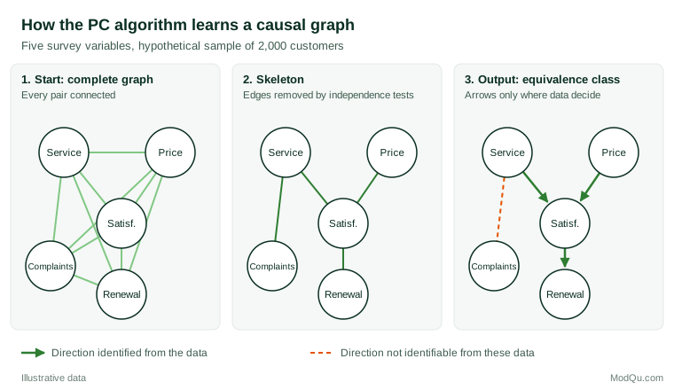
PC proceeds as follows (Figure 1):
- Unconditional tests. Service and price are unrelated, so that edge is removed. Price and complaints are also unrelated.
- Conditional tests. Service and renewal are associated, but independent given satisfaction, so that edge goes. The same applies to price and renewal, to satisfaction and complaints given service, and to renewal and complaints. Four edges remain.
- Colliders. Service and price are not adjacent, and the set that separated them did not include satisfaction. Satisfaction is therefore a collider: service → satisfaction ← price.
- Propagation. Because service points into satisfaction and service is not adjacent to renewal, the edge satisfaction–renewal must point towards renewal. Any other direction would create a collider the data did not show.
The edge between service and complaints stays undirected. Poor service could generate complaints, or complaints could colour later ratings of service, and these data cannot separate the two. That finding tells the research team that a design feature, such as the timing of measurement, is needed.
Practical guidance for survey and business data
- Add background knowledge. Most software lets analysts forbid or require edges. Temporal order is the most useful source: a purchase recorded after the survey cannot cause the survey answers. Such constraints reduce errors and orient more edges (Malinsky & Danks, 2018).
- Treat output as hypotheses. Discovery results are best used to choose which relationships to test in an experiment or a better-designed observational study. A study of cellular signalling showed the value of this approach: learned network structure recovered most known connections and suggested new ones that were then tested experimentally (Sachs et al., 2005).
- Check stability. Rerun the algorithm on bootstrap samples, with different significance levels and with more than one method. Report how often each edge appears rather than one graph.
- Estimate effects with uncertainty about the graph. When several graphs are equally compatible with the data, the IDA approach computes the causal effect under each member of the equivalence class and reports the range (Maathuis et al., 2009).
- Mind the measurement. A noisy measure of a cause does not fully screen off its effects, which can create spurious edges. Ordinal items and weighted samples also need suitable tests.
Limitations and common mistakes
- Assuming faithfulness holds comfortably. Near-cancellations make dependencies too weak to detect in finite samples. Uhler et al. (2013) showed that distributions close to violating faithfulness are far more common than the exact-violation argument suggests, which limits how reliably constraint-based methods work in practice.
- Ignoring hidden confounders. Running PC on survey data where unmeasured attitudes drive many items will produce arrows that reflect common causes. FCI or explicit latent-variable models are safer.
- Conditioning on a selected sample. If the sample contains only current customers or only people who completed a long questionnaire, selection itself can induce associations.
- Reading undirected edges as directed. Plotting software sometimes draws arbitrary arrows on undirected edges. Always check the edge marks.
- Treating the graph as proven. A discovery algorithm is a principled way to search, not a substitute for design (Heinze-Deml et al., 2018).
Key takeaways
Causal discovery algorithms learn what they can about causal structure from patterns of conditional independence and, in some methods, from the shape of the data distribution. Constraint-based methods such as PC, score-based methods such as GES, latent-variable methods such as FCI and non-Gaussian methods such as LiNGAM each rest on explicit assumptions (Glymour et al., 2019). Their honest output is usually a class of graphs rather than a single answer. In survey and business research they are most valuable for generating and prioritising causal hypotheses, especially when combined with background knowledge, stability checks and follow-up experiments.
References
Chickering, D. M. (2002). Optimal structure identification with greedy search. Journal of Machine Learning Research, 3, 507–554.
Glymour, C., Zhang, K., & Spirtes, P. (2019). Review of causal discovery methods based on graphical models. Frontiers in Genetics, 10, Article 524. https://doi.org/10.3389/fgene.2019.00524
Greenland, S., Pearl, J., & Robins, J. M. (1999). Causal diagrams for epidemiologic research. Epidemiology, 10(1), 37–48. https://doi.org/10.1097/00001648-199901000-00008
Heckerman, D., Geiger, D., & Chickering, D. M. (1995). Learning Bayesian networks: The combination of knowledge and statistical data. Machine Learning, 20(3), 197–243. https://doi.org/10.1007/BF00994016
Heinze-Deml, C., Maathuis, M. H., & Meinshausen, N. (2018). Causal structure learning. Annual Review of Statistics and Its Application, 5(1), 371–391. https://doi.org/10.1146/annurev-statistics-031017-100630
Kalisch, M., & Bühlmann, P. (2007). Estimating high-dimensional directed acyclic graphs with the PC-algorithm. Journal of Machine Learning Research, 8, 613–636.
Maathuis, M. H., Kalisch, M., & Bühlmann, P. (2009). Estimating high-dimensional intervention effects from observational data. The Annals of Statistics, 37(6A), 3133–3164. https://doi.org/10.1214/09-AOS685
Malinsky, D., & Danks, D. (2018). Causal discovery algorithms: A practical guide. Philosophy Compass, 13(1), Article e12470. https://doi.org/10.1111/phc3.12470
Pearl, J. (2009). Causality: Models, reasoning, and inference (2nd ed.). Cambridge University Press. https://doi.org/10.1017/CBO9780511803161
Peters, J., Janzing, D., & Schölkopf, B. (2017). Elements of causal inference: Foundations and learning algorithms. MIT Press.
Sachs, K., Perez, O., Pe'er, D., Lauffenburger, D. A., & Nolan, G. P. (2005). Causal protein-signaling networks derived from multiparameter single-cell data. Science, 308(5721), 523–529. https://doi.org/10.1126/science.1105809
Shimizu, S., Hoyer, P. O., Hyvärinen, A., & Kerminen, A. (2006). A linear non-Gaussian acyclic model for causal discovery. Journal of Machine Learning Research, 7, 2003–2030.
Spirtes, P., & Glymour, C. (1991). An algorithm for fast recovery of sparse causal graphs. Social Science Computer Review, 9(1), 62–72. https://doi.org/10.1177/089443939100900106
Spirtes, P., Glymour, C., & Scheines, R. (2000). Causation, prediction, and search (2nd ed.). MIT Press. https://doi.org/10.7551/mitpress/1754.001.0001
Uhler, C., Raskutti, G., Bühlmann, P., & Yu, B. (2013). Geometry of the faithfulness assumption in causal inference. The Annals of Statistics, 41(2), 436–463. https://doi.org/10.1214/12-AOS1080
Zhang, J. (2008). On the completeness of orientation rules for causal discovery in the presence of latent confounders and selection bias. Artificial Intelligence, 172(16–17), 1873–1896. https://doi.org/10.1016/j.artint.2008.08.001