
Statistics · Causal inference
Marginal Structural Models for Time-Varying Confounding
Why ordinary regression fails when treatments and confounders change over time, and how marginal structural models use inverse probability weights to estimate the effect of a treatment strategy.
Many business interventions are not one-off decisions. A retention team offers discounts month after month, and a clinic changes a patient's medication at each visit. In each case, the decision at every point depends on how the customer or patient is doing, and the decision itself changes how they do next. Marginal structural models (MSMs), introduced by Robins and colleagues, are designed for exactly this situation (Robins et al., 2000).
The problem: confounders that are also mediators
Consider a hypothetical subscription business that offers discounts to customers whose engagement is falling. Engagement in month 1 influences who receives a discount in month 1. The discount then raises engagement in month 2, which influences the month 2 discount decision and also predicts renewal directly (Figure 1).
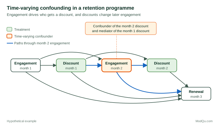
Month 2 engagement is now two things at once. It is a confounder of the month 2 discount, because it affects both that decision and renewal. It is also a mediator of the month 1 discount, because part of that discount's effect on renewal works through engagement. Robins (1986) showed that standard methods cannot handle this structure:
- If the analyst leaves month 2 engagement out of a regression, the estimate is confounded.
- If the analyst includes it, the regression blocks part of the effect of the earlier discount and, when unmeasured factors also affect engagement and renewal, it can open a non-causal path through a collider (Daniel et al., 2013).
Either way, the estimated effect of the discount programme is biased. The problem arises wherever treatment adapts to a changing state, and more covariates do not solve it (Mansournia et al., 2017).
The idea: reweight to remove the feedback
An MSM separates two tasks. First, it builds a weight for each person that removes the link between the time-varying confounders and the treatment received. Second, it fits a simple model for the outcome in the weighted data, with treatment history as the only explanatory variable apart from baseline covariates.
The weights are inverse probability of treatment weights, extending to repeated decisions the logic that Horvitz and Thompson (1952) used for unequal selection probabilities in surveys. Each person is weighted by the inverse of the probability of receiving the treatment history they actually received, given their past. In practice analysts use stabilised weights, which put the probability of treatment given past treatment alone in the numerator (Robins et al., 2000):
SWi = ∏t P(At | Āt−1) ÷ P(At | Āt−1, L̄t)
Here At is treatment at time t, Āt−1 is the treatment history up to the previous period and L̄t is the history of time-varying confounders. In the weighted "pseudo-population", treatment at each time is no longer related to past confounders, so a simple outcome model estimates the causal effect of the treatment strategy. A typical MSM might be:
logit P(Yā = 1) = β0 + β1 × (number of months discounted)
where Yā is the potential outcome under treatment history ā. The model is "marginal" because it describes the population average, and "structural" because it concerns counterfactual outcomes rather than observed associations.
A worked example
Suppose, in illustrative figures, that 40% of customers who received a discount in month 1 also receive one in month 2. Among them, a customer with low engagement has an 80% chance of a month 2 discount, while one with high engagement has only a 10% chance. If a low-engagement customer receives the discount, the month 2 factor of the weight is 0.40 ÷ 0.80 = 0.5: such customers are over-represented among the treated, so each counts for less. A high-engagement customer who receives the discount gets 0.40 ÷ 0.10 = 4.0, standing in for the many similar customers who were not treated. Multiplying the factors across months gives each customer's weight. The weighted renewal model then compares treatment strategies as if discounts had been assigned without regard to engagement.
The classic application estimated the effect of zidovudine on survival in men with HIV. Treatment was started when patients' immune markers worsened, and treatment then improved those markers. Standard time-dependent regression made the drug look harmful, whereas the MSM suggested a protective effect (Hernán et al., 2000).
Practical guidance
- Model treatment carefully. The weights are only as good as the treatment models. Include all variables that drive treatment decisions and predict the outcome, and use flexible functional forms.
- Check the weights. Stabilised weights should have a mean close to 1. Very large weights signal near-violations of positivity, meaning some people almost never receive one of the treatments. Report their distribution and consider truncation at, say, the 1st and 99th percentiles, while noting the bias–variance trade-off involved (Cole & Hernán, 2008).
- Weight for censoring too. Customers who drop out of the data are rarely a random subset. Censoring weights, built in the same way, correct for informative loss to follow-up (Robins et al., 2000).
- Use robust standard errors or the bootstrap, because the weights are estimated (Austin & Stuart, 2015).
- Define the strategy and time zero clearly, as in the target trial framework (Hernán & Robins, 2016).
Limitations
MSMs rely on three conditions: no unmeasured confounding at each time, positivity and correct specification of the treatment models (Hernán & Robins, 2020). None can be confirmed from the data alone. Extreme weights can make estimates unstable, and with rare treatment patterns the effective sample size shrinks quickly. Alternatives such as the parametric g-formula and g-estimation of structural nested models address the same problem with different trade-offs (Daniel et al., 2013).
Key takeaways
When treatments respond to a changing state that they also affect, ordinary regression cannot estimate their effect without bias. Marginal structural models solve this by weighting each person by the inverse probability of their treatment history and then fitting a simple model to the reweighted data. With careful treatment models and weight diagnostics, they let analysts evaluate ongoing programmes as if they had been randomised.
References
Austin, P. C., & Stuart, E. A. (2015). Moving towards best practice when using inverse probability of treatment weighting (IPTW) using the propensity score to estimate causal treatment effects in observational studies. Statistics in Medicine, 34(28), 3661–3679. https://doi.org/10.1002/sim.6607
Cole, S. R., & Hernán, M. A. (2008). Constructing inverse probability weights for marginal structural models. American Journal of Epidemiology, 168(6), 656–664. https://doi.org/10.1093/aje/kwn164
Daniel, R. M., Cousens, S. N., De Stavola, B. L., Kenward, M. G., & Sterne, J. A. C. (2013). Methods for dealing with time-dependent confounding. Statistics in Medicine, 32(9), 1584–1618. https://doi.org/10.1002/sim.5686
Hernán, M. A., Brumback, B., & Robins, J. M. (2000). Marginal structural models to estimate the causal effect of zidovudine on the survival of HIV-positive men. Epidemiology, 11(5), 561–570. https://doi.org/10.1097/00001648-200009000-00012
Hernán, M. A., & Robins, J. M. (2016). Using big data to emulate a target trial when a randomized trial is not available. American Journal of Epidemiology, 183(8), 758–764. https://doi.org/10.1093/aje/kwv254
Hernán, M. A., & Robins, J. M. (2020). Causal inference: What if. Chapman & Hall/CRC.
Horvitz, D. G., & Thompson, D. J. (1952). A generalization of sampling without replacement from a finite universe. Journal of the American Statistical Association, 47(260), 663–685. https://doi.org/10.1080/01621459.1952.10483446
Mansournia, M. A., Etminan, M., Danaei, G., Kaufman, J. S., & Collins, G. (2017). Handling time varying confounding in observational research. BMJ, 359, Article j4587. https://doi.org/10.1136/bmj.j4587
Robins, J. (1986). A new approach to causal inference in mortality studies with a sustained exposure period: Application to control of the healthy worker survivor effect. Mathematical Modelling, 7(9–12), 1393–1512. https://doi.org/10.1016/0270-0255(86)90088-6
Robins, J. M., Hernán, M. A., & Brumback, B. (2000). Marginal structural models and causal inference in epidemiology. Epidemiology, 11(5), 550–560. https://doi.org/10.1097/00001648-200009000-00011