
Statistics · Causal inference
Difference-in-Differences Designs with Multiple Periods and Groups
Why the familiar two-way fixed effects regression can mislead when a policy or product is rolled out at different times, and which newer difference-in-differences estimators to use instead.
Difference-in-differences (DiD) is one of the most widely used methods for estimating the effect of a change that was not randomly assigned. In its classic form, it compares the change in an outcome for a group that was affected, such as stores that adopted a new layout, with the change for a group that was not, over the same before and after periods. Card and Krueger (1994) used this design to study a minimum wage increase in New Jersey, comparing fast-food employment there with neighbouring Pennsylvania. The key assumption is parallel trends: without the change, both groups would have followed the same path.
Real rollouts are rarely so tidy. A retailer introduces self-checkout in some regions in spring, others in autumn, and the rest the following year. States adopt laws in different years. Customers sign up for a programme at different times. This is staggered adoption, with many groups and many periods. Recent research has shown that the standard way of analysing such data can give seriously wrong answers.
The problem with two-way fixed effects
The traditional approach fits a regression with unit fixed effects, time fixed effects and a treatment indicator, often called two-way fixed effects (TWFE) (Angrist & Pischke, 2009). With two groups and two periods, it reproduces the classic DiD estimate. With staggered timing, Goodman-Bacon (2021) showed that the TWFE coefficient is a weighted average of every possible two-group, two-period comparison in the data, including comparisons that use already-treated units as controls for later-treated ones. When treatment effects change over time, those "forbidden" comparisons subtract part of the effect, and some weights can even be negative. de Chaisemartin and D'Haultfœuille (2020) reached a similar conclusion, showing that the estimate can have the opposite sign to every unit's true effect.
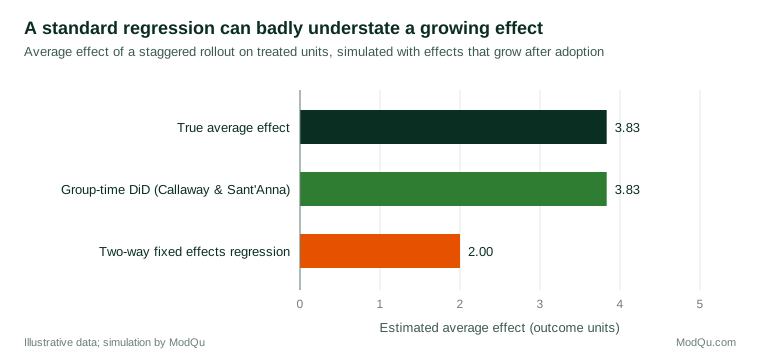
Figure 1 shows the size of the problem in a simple simulation. Two groups adopt a programme at different times and a third never does; the effect grows by one unit each period after adoption. The true average effect on treated units is 3.83. A TWFE regression estimates only 2.00.
Better estimators
The solution is to build the overall estimate from clean comparisons. Callaway and Sant'Anna (2021) estimate a separate effect for each adoption cohort g in each period t, the group-time average treatment effect, comparing cohort g with units that are never treated or not yet treated, relative to the period just before g adopted. These building blocks can then be averaged into an overall effect, an effect by cohort or an event-study profile showing how effects evolve with time since adoption. Sun and Abraham (2021) proposed an interaction-weighted estimator that achieves the same for event-study regressions, avoiding contamination of the pre-period coefficients by effects from other periods. Roth et al. (2023) review these and related methods.
A worked example
Consider a hypothetical chain of 300 stores that introduced a loyalty app in three waves: 80 stores in quarter 3, 120 in quarter 6 and 100 not yet by quarter 10. A TWFE regression of quarterly sales per store on an app indicator estimates an effect of 1.1%. The group-time approach, using the 100 not-yet-adopting stores as controls, shows effects of about 1% in the first quarter after launch rising to 4% after a year, as customers gradually install the app. The aggregated average effect is 2.6%. The TWFE figure was too low because the early stores, whose gains were still growing, were used as controls for the second wave. The event-study profile also tells the business something the single number hides: the app takes about a year to reach its full effect.
Checking and stretching parallel trends
With many periods, analysts can examine pre-adoption trends. Flat event-study coefficients before adoption are reassuring, but pre-tests have low power and conditioning on passing them can bias results. Rambachan and Roth (2023) propose a sensitivity analysis that asks how far post-adoption trends would need to diverge from pre-adoption trends to overturn the conclusion.
Practical guidance
- Plot adoption timing for every unit before estimating anything.
- Avoid plain TWFE when timing varies and effects may change over time; use group-time or interaction-weighted estimators.
- Choose the comparison group deliberately: never-treated units, not-yet-treated units, or both, and say which.
- Report event-study profiles, not just one number, and apply sensitivity analysis to parallel trends.
- Watch for anticipation, such as customers changing behaviour once a rollout is announced.
Key takeaways
Difference-in-differences remains a powerful design for learning from non-random rollouts, but with multiple groups and periods the standard regression can mix good and bad comparisons. Modern estimators that build the answer from clean group-time comparisons, together with honest checks of parallel trends, give estimates of staggered changes that decision-makers can rely on.
References
Angrist, J. D., & Pischke, J.-S. (2009). Mostly harmless econometrics: An empiricist's companion. Princeton University Press. https://doi.org/10.1515/9781400829828
Callaway, B., & Sant'Anna, P. H. C. (2021). Difference-in-differences with multiple time periods. Journal of Econometrics, 225(2), 200–230. https://doi.org/10.1016/j.jeconom.2020.12.001
Card, D., & Krueger, A. B. (1994). Minimum wages and employment: A case study of the fast-food industry in New Jersey and Pennsylvania. The American Economic Review, 84(4), 772–793.
de Chaisemartin, C., & D'Haultfœuille, X. (2020). Two-way fixed effects estimators with heterogeneous treatment effects. American Economic Review, 110(9), 2964–2996. https://doi.org/10.1257/aer.20181169
Goodman-Bacon, A. (2021). Difference-in-differences with variation in treatment timing. Journal of Econometrics, 225(2), 254–277. https://doi.org/10.1016/j.jeconom.2021.03.014
Rambachan, A., & Roth, J. (2023). A more credible approach to parallel trends. The Review of Economic Studies, 90(5), 2555–2591. https://doi.org/10.1093/restud/rdad018
Roth, J., Sant'Anna, P. H. C., Bilinski, A., & Poe, J. (2023). What's trending in difference-in-differences? A synthesis of the recent econometrics literature. Journal of Econometrics, 235(2), 2218–2244. https://doi.org/10.1016/j.jeconom.2023.03.008
Sun, L., & Abraham, S. (2021). Estimating dynamic treatment effects in event studies with heterogeneous treatment effects. Journal of Econometrics, 225(2), 175–199. https://doi.org/10.1016/j.jeconom.2020.09.006