
Statistics · Tests and models
Structural Equation Modelling
How structural equation modelling links survey items to latent constructs and tests the paths between them, how to judge model fit, and which pitfalls to avoid in market research.
Many of the things businesses most want to understand cannot be observed directly. Satisfaction, trust, perceived value, brand attachment and loyalty are constructs: ideas that we infer from the way people answer several related survey questions. Structural equation modelling (SEM) is a family of methods designed for exactly this situation. It combines two ideas in one model: a measurement model, which links each unobserved construct to the questions that measure it, and a structural model, which describes how the constructs relate to one another (Bollen, 1989; Kline, 2016).
This article explains what SEM does, how it differs from running a series of regressions on averaged scale scores, how to read a fitted model, and where the method is most often misused. It is aimed at analysts and decision-makers who meet SEM results in customer experience, brand tracking and employee research and want to judge them with confidence.
From path analysis to latent variables
SEM has two roots. The first is path analysis, introduced by the geneticist Sewall Wright (1921), who represented a set of hypothesised causal links as a diagram of arrows and showed how the correlations among observed variables could be decomposed into the contributions of each path. The second is factor analysis, which explains the correlations among many observed variables by a smaller number of unobserved common factors. Jöreskog (1970) brought the two together in a general method for the analysis of covariance structures, estimated by maximum likelihood, which became the basis of the LISREL software and of most modern SEM programs.
The key insight is that a theory about constructs implies a particular pattern of variances and covariances among the survey items. If the theory is right, the covariance matrix predicted by the model should be close to the covariance matrix observed in the data. SEM estimates the model's parameters by making the two matrices as similar as possible, and then asks how large the remaining discrepancy is.
The two parts of a structural equation model
The measurement model
In the measurement model, each latent variable is measured by several observed indicators, usually survey items. Each item is written as:
xi = λiξ + δi
where ξ is the latent variable, λi is the item's factor loading and δi is the item's unique part, which includes measurement error. Fitting the measurement model on its own is a confirmatory factor analysis (CFA). The loadings show how strongly each item reflects its construct, and the error terms absorb the part of each answer that is specific to that question or simply noise.
The structural model
The structural model specifies the regressions among the latent variables themselves. In a simple customer model it might read:
η1 = γ1ξ + ζ1 and η2 = β21η1 + γ2ξ + ζ2
where ξ is an exogenous construct (one that is not explained in the model), η1 and η2 are endogenous constructs, the γ and β terms are path coefficients, and the ζ terms are disturbances that capture everything the model does not explain. Because the paths link latent variables rather than error-laden averages, the estimated relationships are corrected for measurement error in the items.
Why not just average the items?
The usual alternative is to average each set of items into a scale score and run ordinary regressions. This is simpler, but it treats the averages as if they were measured without error. Random measurement error weakens correlations, a problem known as attenuation, so regression coefficients based on scale scores tend to be biased towards zero for the predictor that is measured poorly, and can be biased in either direction for the other predictors in the model. SEM models measurement error explicitly, so the structural paths are estimated between the constructs themselves.
SEM also brings three practical advantages. It estimates several equations at once, so a construct can be an outcome in one equation and a predictor in another. It produces direct, indirect and total effects in a single analysis. And it provides tests of whether the whole set of assumptions is consistent with the data, rather than judging each equation in isolation.
A worked example: service quality, satisfaction and loyalty
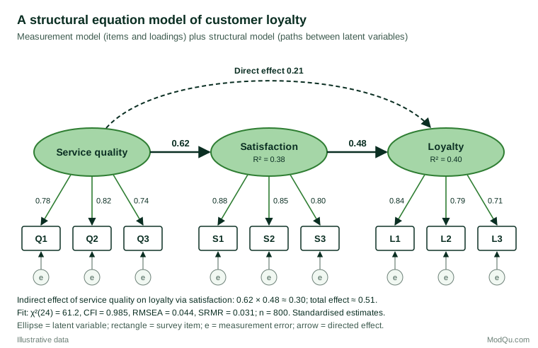
Consider a hypothetical survey of 800 customers of a subscription service. Three constructs are each measured by three agreement items on a seven-point scale: service quality (Q1 to Q3, for example "Staff resolve my problems quickly"), satisfaction (S1 to S3) and loyalty (L1 to L3, including intention to renew and willingness to recommend). The theory is that service quality raises satisfaction, satisfaction raises loyalty, and quality may also have a direct effect on loyalty. This structure is a simplified version of the cause-and-effect logic behind national customer satisfaction indices, which link perceived quality and value to satisfaction and then to complaints and loyalty (Fornell et al., 1996).
Step 1: check the measurement model
Following the two-step approach recommended by Anderson and Gerbing (1988), the analyst first fits the measurement model as a CFA, allowing the three constructs to correlate freely, and only then adds the structural paths. This separates two questions: do the items measure the constructs they were written for, and are the constructs related as the theory says? If the measurement model fits poorly, the structural results cannot be trusted.
In the illustrative data, all standardised loadings lie between 0.71 and 0.88. Two summary measures are commonly reported for each construct. The average variance extracted (AVE) is the mean of the squared standardised loadings; for service quality it is (0.78² + 0.82² + 0.74²) ÷ 3 ≈ 0.61, meaning the construct accounts for about 61% of the variance of its items on average. Composite reliability is about 0.82 for service quality, 0.88 for satisfaction and 0.82 for loyalty. Fornell and Larcker (1981) proposed that an AVE of at least 0.5 indicates adequate convergent validity, and that discriminant validity is supported when each construct's AVE exceeds its squared correlation with every other construct. Later work has shown that this criterion can miss real discriminant validity problems, and that the heterotrait–monotrait ratio of correlations is more sensitive (Henseler et al., 2015).
Step 2: estimate the structural model
The standardised path from service quality to satisfaction is 0.62, from satisfaction to loyalty 0.48, and the direct path from quality to loyalty 0.21. The model explains 38% of the variance in satisfaction and 40% in loyalty. The indirect effect of quality on loyalty through satisfaction is the product of the two paths, 0.62 × 0.48 ≈ 0.30, so the total effect is about 0.21 + 0.30 = 0.51. In words: in this hypothetical model, most of the association between service quality and loyalty runs through satisfaction, but not all of it.
Indirect effects need appropriate tests. The traditional causal-steps approach checks a sequence of separate regressions, but it does not test the indirect effect itself. Preacher and Hayes (2008) recommend estimating the indirect effect directly and using a bootstrap confidence interval, because the sampling distribution of a product of two coefficients is usually skewed. SEM software makes this straightforward.
Step 3: judge overall fit
The illustrative model has 45 distinct variances and covariances among the nine items and 21 free parameters, leaving 24 degrees of freedom. The fit statistics are χ²(24) = 61.2, p < 0.001; comparative fit index (CFI) = 0.985; root mean square error of approximation (RMSEA) = 0.044; and standardised root mean square residual (SRMR) = 0.031. How to read these numbers is the subject of the next section.
Judging model fit
The chi-square test
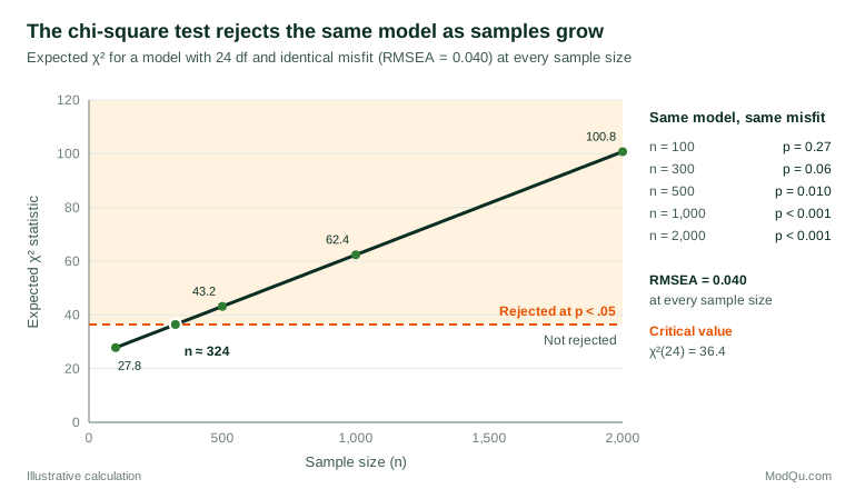
The model chi-square tests the null hypothesis that the model reproduces the population covariance matrix exactly. It is the only formal test of fit, but it has two well-known limitations. First, no model of real behaviour is exactly true, so the null hypothesis is almost always false. Second, the statistic grows with sample size for any fixed amount of misfit. A small, practically unimportant discrepancy will be "significant" in a large survey, which is exactly what Figure 2 shows. The chi-square should still be reported, and a significant result is a prompt to look for the source of misfit, but it should not be the only basis for accepting or rejecting a model.
Approximate fit indices
Because of these limitations, analysts also report approximate fit indices that describe how large the misfit is rather than whether it is exactly zero:
- RMSEA estimates misfit per degree of freedom in the population and comes with a confidence interval. Browne and Cudeck (1992) suggested that values of about 0.05 or less indicate close fit, values up to about 0.08 a reasonable error of approximation, and that models above 0.10 should not be used.
- CFI compares the fitted model with a baseline model in which all items are uncorrelated, and ranges from 0 to 1 (Bentler, 1990).
- SRMR is the average difference between observed and model-implied correlations.
Hu and Bentler (1999) used simulations to propose combinations of cut-offs, such as CFI close to 0.95 or above, RMSEA close to 0.06 or below and SRMR close to 0.08 or below. These values are now widely treated as pass marks, which their authors did not intend. Marsh et al. (2004) warned against turning them into "golden rules", because the behaviour of fit indices depends on the number of items, the size of the loadings and the type of misspecification. Fit indices are best used as one piece of evidence alongside inspection of residuals, the size and sense of the estimates, and comparison with plausible alternative models.
Good fit is not proof
A well-fitting model is consistent with the data, but so are other models. MacCallum et al. (1993) showed that many models have equivalent models: alternatives with different, sometimes reversed, paths that fit any data set exactly as well. In the example, a model in which loyalty drives satisfaction would fit just as well as one in which satisfaction drives loyalty. Tomarken and Waller (2003) add that a model can fit well overall while containing serious local errors, or while explaining very little of the variance in the outcomes. Fit tells you whether the model's assumptions are contradicted by the data; it cannot tell you that the assumed direction of influence is the right one.
SEM and causality
SEM is sometimes called "causal modelling", and its path diagrams look like causal claims. The arrows do encode causal assumptions, and so do the arrows that are left out: every missing path is a claim that there is no direct effect (Pearl, 2009). But the method does not create causal evidence that the design does not contain. With cross-sectional survey data, the order of the variables is assumed by the analyst, not observed, and omitted common causes can produce associations that look like effects. MacCallum and Austin (2000), reviewing published applications in psychology, noted that directional claims were often made from cross-sectional data and that equivalent models were seldom acknowledged.
For business use, SEM results are best presented as estimates under a stated theory: "if the model is right, a one standard deviation improvement in perceived service quality is associated with about half a standard deviation higher loyalty, mostly through satisfaction." Stronger causal claims need stronger designs, such as experiments, longitudinal panels in which the cause is measured before the effect, or natural variation that can be argued to be as good as random.
Practical guidance for survey and business data
Know when SEM adds value
SEM is most useful when the constructs of interest are measured by several items each, when the theory involves chains of influence such as quality affecting satisfaction and satisfaction affecting loyalty, and when the question is about the relationships between constructs rather than the prediction of a single outcome. For a one-off driver analysis of a single overall rating, a well-specified regression may answer the business question just as well and is easier to explain. The extra effort pays off when the same model will be tracked over time or compared across markets.
Design the measurement before you collect data
- Use at least three good items per construct. Constructs with one or two indicators are hard to identify and estimate. Write items that clearly reflect a single idea and avoid near-duplicate wording, which can inflate loadings without adding information.
- Plan for common method variance. When predictors and outcomes come from the same respondent, in the same questionnaire and with the same response format, shared method effects can inflate the relationships between constructs. Podsakoff et al. (2003) review the procedural remedies (separating measures in time or source, varying scale formats, protecting anonymity) and the statistical ones.
Choose the right estimator
- Ordinal items. Most survey items are ordinal rating scales. Rhemtulla et al. (2012) found that with five or more response categories, robust maximum likelihood treating the items as continuous generally performs acceptably, while with fewer categories, estimators designed for categorical data are preferable.
- Non-normal data. Skewed answers distort the standard chi-square test and standard errors. Curran et al. (1996) showed that the maximum likelihood chi-square becomes too large under non-normality and that a scaled (Satorra–Bentler) statistic performs much better.
- Missing data. Full information maximum likelihood uses all the available answers from each respondent. In simulations it outperformed listwise and pairwise deletion when data were missing at random (Enders & Bandalos, 2001).
- Weights and clustering. For weighted or clustered samples, use estimators and standard errors that account for the design, which most SEM software now provides.
Get enough data
There is no universal minimum sample size. Wolf et al. (2013) found in simulations that the sample needed for adequate power, low bias and admissible solutions ranged from 30 to 460 cases across the models they examined, depending on the number of factors, the number of indicators and the strength of the loadings. Weak loadings, many constructs, small effects and complex mediation chains all raise the requirement. A simulation-based power analysis for the specific model is better than any rule of thumb.
Report transparently
Report the full model (ideally the diagram), the estimator, how missing data were handled, all loadings and paths with standard errors or confidence intervals, R² for each outcome, the chi-square with its degrees of freedom and at least two approximate fit indices. Open-source software such as the lavaan package for R makes models easy to share and reproduce (Rosseel, 2012), and standard texts set out what to report (Kline, 2016).
Covariance-based or variance-based SEM?
The approach described so far is covariance-based SEM. Partial least squares SEM (PLS-SEM) is a variance-based alternative that builds weighted composites of the items and maximises the explained variance of the outcomes. It is popular in marketing and information systems research, and Hair et al. (2011) argue that it suits prediction-oriented work, complex models and smaller samples. It does not offer the same global test of model fit, and its composites do not fully remove measurement error, so the choice should follow the purpose of the analysis: testing a theory about constructs favours covariance-based SEM, while building a predictive index may favour PLS-SEM.
Common mistakes
- Modifying the model until it fits. Software suggests "modification indices": parameters that would most improve fit if freed. Adding them one by one, driven by the data rather than theory, capitalises on chance. MacCallum et al. (1992) showed that such data-driven modifications often fail to replicate in new samples. Any modifications should be theoretically justified, reported, and ideally tested on a holdout sample.
- Treating fit cut-offs as pass marks. A model that just clears a CFI of 0.95 is not automatically valid, and one that falls slightly short is not automatically wrong (Marsh et al., 2004).
- Ignoring the measurement model. Interpreting structural paths before confirming that the items measure the intended constructs reverses the logic of the two-step approach (Anderson & Gerbing, 1988).
- Reading arrows as proven causes. Path coefficients from cross-sectional data are conditional associations under the analyst's assumptions, not demonstrated effects.
- Comparing groups without testing measurement invariance. Before comparing path coefficients or latent means across countries, segments or survey modes, test whether the items work the same way in each group; otherwise differences may reflect the questions rather than the people.
- Over-complex models for the sample. Large models with many constructs and small samples produce unstable estimates, improper solutions such as negative error variances, and fit indices that are hard to interpret (Wolf et al., 2013).
Key takeaways
Structural equation modelling combines measurement and explanation in one framework. It links survey items to the constructs they are meant to capture, corrects the relationships between constructs for measurement error, and estimates direct, indirect and total effects in a single model. Used well, it turns a battery of rating questions into a coherent, testable account of how customers or employees think.
Its strengths depend on discipline. Check the measurement model first, choose estimators suited to ordinal and incomplete survey data, judge fit with several indices and with judgement rather than fixed cut-offs, consider equivalent models, and resist modifying the model until it fits. Above all, remember that SEM tests whether a theory is consistent with the data; it does not, by itself, prove that the theory is true.
References
Anderson, J. C., & Gerbing, D. W. (1988). Structural equation modeling in practice: A review and recommended two-step approach. Psychological Bulletin, 103(3), 411–423. https://doi.org/10.1037/0033-2909.103.3.411
Bentler, P. M. (1990). Comparative fit indexes in structural models. Psychological Bulletin, 107(2), 238–246. https://doi.org/10.1037/0033-2909.107.2.238
Bollen, K. A. (1989). Structural equations with latent variables. Wiley. https://doi.org/10.1002/9781118619179
Browne, M. W., & Cudeck, R. (1992). Alternative ways of assessing model fit. Sociological Methods & Research, 21(2), 230–258. https://doi.org/10.1177/0049124192021002005
Curran, P. J., West, S. G., & Finch, J. F. (1996). The robustness of test statistics to nonnormality and specification error in confirmatory factor analysis. Psychological Methods, 1(1), 16–29. https://doi.org/10.1037/1082-989X.1.1.16
Enders, C. K., & Bandalos, D. L. (2001). The relative performance of full information maximum likelihood estimation for missing data in structural equation models. Structural Equation Modeling: A Multidisciplinary Journal, 8(3), 430–457. https://doi.org/10.1207/S15328007SEM0803_5
Fornell, C., Johnson, M. D., Anderson, E. W., Cha, J., & Bryant, B. E. (1996). The American Customer Satisfaction Index: Nature, purpose, and findings. Journal of Marketing, 60(4), 7–18. https://doi.org/10.1177/002224299606000403
Fornell, C., & Larcker, D. F. (1981). Evaluating structural equation models with unobservable variables and measurement error. Journal of Marketing Research, 18(1), 39–50. https://doi.org/10.1177/002224378101800104
Hair, J. F., Ringle, C. M., & Sarstedt, M. (2011). PLS-SEM: Indeed a silver bullet. Journal of Marketing Theory and Practice, 19(2), 139–152. https://doi.org/10.2753/MTP1069-6679190202
Henseler, J., Ringle, C. M., & Sarstedt, M. (2015). A new criterion for assessing discriminant validity in variance-based structural equation modeling. Journal of the Academy of Marketing Science, 43(1), 115–135. https://doi.org/10.1007/s11747-014-0403-8
Hu, L., & Bentler, P. M. (1999). Cutoff criteria for fit indexes in covariance structure analysis: Conventional criteria versus new alternatives. Structural Equation Modeling: A Multidisciplinary Journal, 6(1), 1–55. https://doi.org/10.1080/10705519909540118
Jöreskog, K. G. (1970). A general method for analysis of covariance structures. Biometrika, 57(2), 239–251. https://doi.org/10.1093/biomet/57.2.239
Kline, R. B. (2016). Principles and practice of structural equation modeling (4th ed.). Guilford Press.
MacCallum, R. C., & Austin, J. T. (2000). Applications of structural equation modeling in psychological research. Annual Review of Psychology, 51, 201–226. https://doi.org/10.1146/annurev.psych.51.1.201
MacCallum, R. C., Roznowski, M., & Necowitz, L. B. (1992). Model modifications in covariance structure analysis: The problem of capitalization on chance. Psychological Bulletin, 111(3), 490–504. https://doi.org/10.1037/0033-2909.111.3.490
MacCallum, R. C., Wegener, D. T., Uchino, B. N., & Fabrigar, L. R. (1993). The problem of equivalent models in applications of covariance structure analysis. Psychological Bulletin, 114(1), 185–199. https://doi.org/10.1037/0033-2909.114.1.185
Marsh, H. W., Hau, K.-T., & Wen, Z. (2004). In search of golden rules: Comment on hypothesis-testing approaches to setting cutoff values for fit indexes and dangers in overgeneralizing Hu and Bentler's (1999) findings. Structural Equation Modeling: A Multidisciplinary Journal, 11(3), 320–341. https://doi.org/10.1207/s15328007sem1103_2
Pearl, J. (2009). Causality: Models, reasoning, and inference (2nd ed.). Cambridge University Press. https://doi.org/10.1017/CBO9780511803161
Podsakoff, P. M., MacKenzie, S. B., Lee, J.-Y., & Podsakoff, N. P. (2003). Common method biases in behavioral research: A critical review of the literature and recommended remedies. Journal of Applied Psychology, 88(5), 879–903. https://doi.org/10.1037/0021-9010.88.5.879
Preacher, K. J., & Hayes, A. F. (2008). Asymptotic and resampling strategies for assessing and comparing indirect effects in multiple mediator models. Behavior Research Methods, 40(3), 879–891. https://doi.org/10.3758/BRM.40.3.879
Rhemtulla, M., Brosseau-Liard, P. É., & Savalei, V. (2012). When can categorical variables be treated as continuous? A comparison of robust continuous and categorical SEM estimation methods under suboptimal conditions. Psychological Methods, 17(3), 354–373. https://doi.org/10.1037/a0029315
Rosseel, Y. (2012). lavaan: An R package for structural equation modeling. Journal of Statistical Software, 48(2), 1–36. https://doi.org/10.18637/jss.v048.i02
Tomarken, A. J., & Waller, N. G. (2003). Potential problems with "well fitting" models. Journal of Abnormal Psychology, 112(4), 578–598. https://doi.org/10.1037/0021-843X.112.4.578
Wolf, E. J., Harrington, K. M., Clark, S. L., & Miller, M. W. (2013). Sample size requirements for structural equation models: An evaluation of power, bias, and solution propriety. Educational and Psychological Measurement, 73(6), 913–934. https://doi.org/10.1177/0013164413495237
Wright, S. (1921). Correlation and causation. Journal of Agricultural Research, 20(7), 557–585.