
Statistics · Tests and models
Multilevel and Hierarchical Models
How multilevel models handle data in which customers sit within stores, employees within teams or answers within respondents, and why they give fairer estimates for small groups.
Business data are rarely a flat list of independent observations. Customers shop at particular stores, employees work in teams, students sit in classes and survey respondents answer many questions each. People in the same group tend to resemble one another. Multilevel models, also called hierarchical, mixed-effects or random-effects models, are regression models built for this nested structure (Raudenbush & Bryk, 2002; Snijders & Bosker, 2012).
Why nesting matters
Ignoring the grouping causes two problems. The first is false precision. If customers of the same branch give similar ratings, 60 interviews in one branch carry less independent information than 60 interviews spread across 60 branches. Kish (1965) captured this with the design effect, which for clustered data is approximately:
Deff ≈ 1 + (m − 1) × ICC
where m is the average number of observations per group and the intraclass correlation (ICC) is the share of total variance that lies between groups. Even a small ICC matters when groups are large. With an ICC of 0.08 and 60 respondents per branch, the design effect is about 5.9, so 2,400 interviews behave like roughly 400 independent ones. Standard errors from an ordinary regression would be far too small.
The second problem is drawing conclusions at the wrong level. A relationship between branch averages need not hold for individual customers, and the reverse is also true. Robinson (1950) showed that correlations computed from aggregated data can differ sharply from the correlation among individuals, an error now known as the ecological fallacy.
The model
A simple two-level model for the satisfaction score of customer i in branch j is:
yij = β0 + uj + β1xij + eij, uj ~ N(0, τ²), eij ~ N(0, σ²)
The overall intercept β0 and slope β1 are fixed effects. Each branch has its own deviation uj, a random effect drawn from a distribution with between-branch variance τ², while σ² is the variance among customers within a branch. The ICC is τ² ÷ (τ² + σ²). The model can be extended with random slopes, letting the effect of x differ by branch, with branch-level predictors such as store size, and with further levels such as branches within regions. Gelman and Hill (2007) give an accessible treatment, and open-source software such as the lme4 package fits these models routinely (Bates et al., 2015).
Partial pooling: a worked example
Suppose a hypothetical retailer surveys 2,400 customers across 40 branches, and the model estimates an overall mean of 7.2, a between-branch standard deviation τ = 0.6 and a within-branch standard deviation σ = 2.0, giving an ICC of about 0.08.
There are two naive ways to estimate a branch's mean. Complete pooling ignores branches and gives everyone 7.2. No pooling uses each branch's raw mean, however few interviews it rests on. A multilevel model takes a weighted compromise, known as partial pooling or shrinkage:
estimatej = λj × ȳj + (1 − λj) × ȳ, where λj = τ² ÷ (τ² + σ² ÷ nj)
Branch A has only 8 respondents and a raw mean of 8.6. Its weight is 0.36 ÷ (0.36 + 4 ÷ 8) = 0.42, so its estimate is 0.42 × 8.6 + 0.58 × 7.2 ≈ 7.8. Branch J has 250 respondents; its weight is 0.96 and its estimate hardly moves from 7.0.
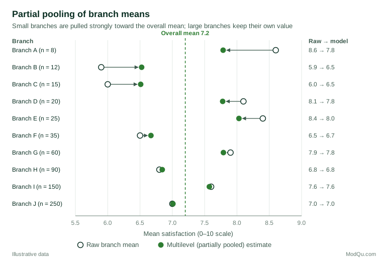
Shrinkage is not a fudge. Extreme raw means from small samples are partly noise, and the next survey wave would usually show them closer to the average. Partial pooling anticipates this regression to the mean and, on average, gives more accurate branch estimates than either extreme (Gelman & Hill, 2007). The same idea powers multilevel regression and poststratification (MRP), which produces estimates for small regions or segments from national samples (Park et al., 2004).
Practical guidance for survey and business data
- Report the ICC. It tells stakeholders how much of the variation in an outcome lies between stores, teams or regions, and therefore how much room there is for group-level action.
- Plan for enough groups. The number of groups matters more than the number of people per group for estimating group-level variance. In simulations by Maas and Hox (2005), regression coefficients and variance components were estimated without bias even with 30 groups, but the standard errors of the group-level variances were biased with 50 or fewer groups.
- Centre predictors deliberately. Centring an individual predictor on its group mean separates the within-group effect from the between-group effect, which answer different business questions (Enders & Tofighi, 2007).
- Use it for league tables. Ranking branches, agents or regions on raw means rewards small units with lucky samples. Shrunken estimates with intervals give a fairer ranking.
- Model repeated measures. Several ratings from the same respondent, or monthly scores from the same customer, are also nested data.
Common mistakes
- Ignoring clustering and reporting significance tests as if every observation were independent.
- Treating groups as fixed when they are a sample. If the branches surveyed stand for a wider set, random effects are the natural choice; fixed dummies suit a small, complete set of groups of direct interest.
- Overcomplicating the random part. Models with many random slopes and few groups often fail to converge or give unstable variance estimates.
- Reading group-level results as individual-level facts, or the reverse.
Key takeaways
Multilevel models respect the way data are actually organised. They give honest standard errors when observations are clustered, separate within-group from between-group effects, and borrow strength across groups so that small units receive sensible estimates. For any survey analysed by store, region, team or wave, they should be the default rather than the exception.
References
Bates, D., Mächler, M., Bolker, B., & Walker, S. (2015). Fitting linear mixed-effects models using lme4. Journal of Statistical Software, 67(1), 1–48. https://doi.org/10.18637/jss.v067.i01
Enders, C. K., & Tofighi, D. (2007). Centering predictor variables in cross-sectional multilevel models: A new look at an old issue. Psychological Methods, 12(2), 121–138. https://doi.org/10.1037/1082-989X.12.2.121
Gelman, A., & Hill, J. (2007). Data analysis using regression and multilevel/hierarchical models. Cambridge University Press. https://doi.org/10.1017/CBO9780511790942
Kish, L. (1965). Survey sampling. Wiley.
Maas, C. J. M., & Hox, J. J. (2005). Sufficient sample sizes for multilevel modeling. Methodology, 1(3), 86–92. https://doi.org/10.1027/1614-2241.1.3.86
Park, D. K., Gelman, A., & Bafumi, J. (2004). Bayesian multilevel estimation with poststratification: State-level estimates from national polls. Political Analysis, 12(4), 375–385. https://doi.org/10.1093/pan/mph024
Raudenbush, S. W., & Bryk, A. S. (2002). Hierarchical linear models: Applications and data analysis methods (2nd ed.). Sage.
Robinson, W. S. (1950). Ecological correlations and the behavior of individuals. American Sociological Review, 15(3), 351–357. https://doi.org/10.2307/2087176
Snijders, T. A. B., & Bosker, R. J. (2012). Multilevel analysis: An introduction to basic and advanced multilevel modeling (2nd ed.). Sage.