
Statistics · Tests and models
Survival Analysis and Time-to-Event Data
How survival analysis measures how long it takes for something to happen, such as a customer cancelling, and why Kaplan–Meier curves and Cox models handle incomplete follow-up correctly.
How long do subscribers stay before cancelling? How many weeks pass before a new customer makes a second purchase? How long does an employee stay after joining? Questions like these concern time-to-event data: the outcome is not just whether something happens, but when. Survival analysis is the family of methods built for such data. Its name comes from medicine, where the event was often death, but the same tools apply to customer churn, product failure, time to repurchase and many other business questions (Kleinbaum & Klein, 2012; Klein & Moeschberger, 2003).
The central problem: censoring
What makes time-to-event data special is that, for some people, the event has not happened yet when the data are analysed. A customer who signed up three months ago and is still active has a lifetime of at least three months, but we do not know how much longer. This is called right censoring, and it is almost always present in business data, because customers join at different times and the analysis takes place on a fixed date.
Ordinary methods handle censoring badly. Dropping censored customers throws away information and biases results toward short lifetimes, because long-lived customers are the ones most likely to be still active. Treating them as if they never had the event, for example by counting everyone still active as "retained", understates the true churn rate. Averaging the time to cancellation among those who have already cancelled gives a figure that is too short, since it ignores everyone who has stayed longer. Survival methods use each customer's information for exactly as long as they were observed.
These methods assume that censoring is non-informative: customers whose follow-up ends are no more or less likely to have the event than those who remain under observation. Censoring because the analysis date arrived usually meets this assumption. Censoring because a customer stopped answering a panel survey, perhaps because they were losing interest, may not (Leung et al., 1997).
Survival and hazard
Two functions describe time-to-event data. The survival function, S(t), is the probability that the event has not happened by time t: the share of customers still subscribed after t months. The hazard function, h(t), is the instantaneous rate at which the event occurs at time t among those who have not yet had it. In churn terms, the hazard at month 6 is the risk of cancelling in month 6 for customers who reached month 6.
The hazard often tells the more useful business story. Many subscription products show a high hazard in the first weeks, as customers who were never a good fit leave, followed by a lower and steadier hazard. Part of this fall can reflect heterogeneity rather than any change in individual customers: high-risk customers leave first, so the remaining group looks more loyal over time (Fader & Hardie, 2007).
Kaplan–Meier estimation
The Kaplan–Meier estimator is the standard way to estimate the survival curve from censored data (Kaplan & Meier, 1958). At each time an event occurs, it computes the proportion of people still at risk who survive that moment, and multiplies these proportions together:
Ŝ(t) = ∏ti ≤ t (1 − di ÷ ni)
where di is the number of events at time ti and ni the number still at risk just before it. Censored customers count in the risk set until the moment they are censored, then leave it without counting as events. The result is a step curve that drops at each event.
A worked example
Consider a hypothetical subscription service that tracks 1,000 customers who joined at different points over two years: 500 joined with an introductory discount and 500 at full price. When the data are extracted, 256 of the discount group and 141 of the full-price group have cancelled; everyone else is censored.
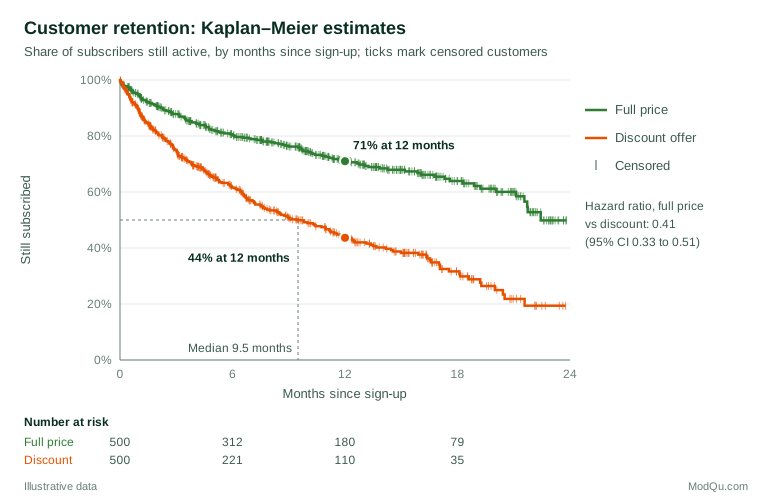
The Kaplan–Meier estimates show that 44% of discount customers are still subscribed after 12 months, against 71% of full-price customers. The median lifetime of the discount group, the time by which half have cancelled, is about 9.5 months. For the full-price group, the median lies beyond 18 months. A naive calculation that simply counts customers seen to cancel within their first 12 months, treating everyone else as retained, would suggest that 45% of the discount group churn within a year. The Kaplan–Meier estimate is 56%, because many customers had not yet been observed for a full year.
The table of numbers at risk is an essential part of the chart. The right-hand end of each curve rests on few customers and is much less certain than the left, so sudden steps late in follow-up should not be over-interpreted (Clark et al., 2003).
Comparing groups: the log-rank test
The log-rank test compares survival curves across groups. At each event time, it compares the number of events observed in each group with the number expected if the groups shared the same survival curve, and combines these comparisons over the whole follow-up (Bland & Altman, 2004). In the example, the test gives a chi-square statistic of about 75 on one degree of freedom (p < 0.001), so a difference this large would be very unlikely if the two groups truly had the same retention.
The Cox proportional hazards model
To estimate the effect of several factors at once, analysts use the Cox proportional hazards model (Cox, 1972). It models the hazard as a baseline hazard, left unspecified, multiplied by a function of the predictors:
h(t | x) = h0(t) × exp(β1x1 + … + βkxk)
Exponentiated coefficients are hazard ratios. In the example, the hazard ratio for full-price versus discount customers is 0.41 (95% confidence interval 0.33 to 0.51): at any point in time, full-price customers cancel at roughly 41% of the rate of discount customers. Further predictors, such as channel, plan size or a satisfaction score from an onboarding survey, can be added in the same way as in other regression models.
The model's key assumption is that hazard ratios are constant over time. If a discount group cancels heavily when the discount expires but then behaves like everyone else, the assumption fails. Plots of scaled residuals and formal tests help check it (Grambsch & Therneau, 1994), and the model can be extended with time-varying effects or stratification when it does not hold (Therneau & Grambsch, 2000).
Beyond the hazard ratio
Hazard ratios are not always the clearest summary. Hernán (2010) pointed out that a hazard ratio averages over a period in which the people at risk change, which complicates causal interpretation, and recommended reporting survival curves as well. The restricted mean survival time (RMST), the area under the survival curve up to a chosen horizon, is an intuitive alternative that remains valid when hazards are not proportional (Royston & Parmar, 2013). In the example, average subscribed time over the first 18 months is about 10.0 months for discount customers and 13.9 months for full-price customers, a gap that translates directly into revenue.
Practical guidance for survey and business data
- Define the clock carefully. State the start event (sign-up, first purchase), the end event (cancellation, lapse) and how censoring is handled.
- Use discrete-time models for interval data. When events are known only to the month or to a survey wave, discrete-time survival models, fitted as logistic regressions on person-period data, are simple and flexible (Singer & Willett, 1993).
- Handle competing risks. A customer who downgrades to a free tier can no longer cancel a paid one. When other events prevent the event of interest, ordinary Kaplan–Meier estimates overstate its probability, and competing-risks methods are needed (Fine & Gray, 1999).
- Link survival to value. Retention curves feed directly into estimates of customer lifetime value, and projecting retention beyond the data requires a model that accounts for differences between customers (Fader & Hardie, 2007).
Common mistakes
- Excluding or ignoring censored cases, which distorts both lifetimes and churn rates.
- Reading late parts of the curve without looking at the numbers at risk.
- Assuming proportional hazards without checking it.
- Conditioning on the future. Classifying customers by something that happens after the start, such as "made a second purchase", gives that group a built-in survival advantage, since they had to stay long enough to make it.
Key takeaways
Survival analysis answers "how long until?" questions while using the information in incomplete follow-up correctly. Kaplan–Meier curves describe retention, the log-rank test compares groups, and the Cox model estimates the effect of several factors as hazard ratios. Report curves with numbers at risk, check the proportional hazards assumption, and consider measures such as restricted mean survival time that speak directly to business value.
References
Bland, J. M., & Altman, D. G. (2004). The logrank test. BMJ, 328(7447), 1073. https://doi.org/10.1136/bmj.328.7447.1073
Clark, T. G., Bradburn, M. J., Love, S. B., & Altman, D. G. (2003). Survival analysis part I: Basic concepts and first analyses. British Journal of Cancer, 89(2), 232–238. https://doi.org/10.1038/sj.bjc.6601118
Cox, D. R. (1972). Regression models and life-tables. Journal of the Royal Statistical Society Series B: Statistical Methodology, 34(2), 187–202. https://doi.org/10.1111/j.2517-6161.1972.tb00899.x
Fader, P. S., & Hardie, B. G. S. (2007). How to project customer retention. Journal of Interactive Marketing, 21(1), 76–90. https://doi.org/10.1002/dir.20074
Fine, J. P., & Gray, R. J. (1999). A proportional hazards model for the subdistribution of a competing risk. Journal of the American Statistical Association, 94(446), 496–509. https://doi.org/10.1080/01621459.1999.10474144
Grambsch, P. M., & Therneau, T. M. (1994). Proportional hazards tests and diagnostics based on weighted residuals. Biometrika, 81(3), 515–526. https://doi.org/10.1093/biomet/81.3.515
Hernán, M. A. (2010). The hazards of hazard ratios. Epidemiology, 21(1), 13–15. https://doi.org/10.1097/EDE.0b013e3181c1ea43
Kaplan, E. L., & Meier, P. (1958). Nonparametric estimation from incomplete observations. Journal of the American Statistical Association, 53(282), 457–481. https://doi.org/10.1080/01621459.1958.10501452
Klein, J. P., & Moeschberger, M. L. (2003). Survival analysis: Techniques for censored and truncated data (2nd ed.). Springer. https://doi.org/10.1007/b97377
Kleinbaum, D. G., & Klein, M. (2012). Survival analysis: A self-learning text (3rd ed.). Springer. https://doi.org/10.1007/978-1-4419-6646-9
Leung, K. M., Elashoff, R. M., & Afifi, A. A. (1997). Censoring issues in survival analysis. Annual Review of Public Health, 18, 83–104. https://doi.org/10.1146/annurev.publhealth.18.1.83
Royston, P., & Parmar, M. K. B. (2013). Restricted mean survival time: An alternative to the hazard ratio for the design and analysis of randomized trials with a time-to-event outcome. BMC Medical Research Methodology, 13, Article 152. https://doi.org/10.1186/1471-2288-13-152
Singer, J. D., & Willett, J. B. (1993). It's about time: Using discrete-time survival analysis to study duration and the timing of events. Journal of Educational Statistics, 18(2), 155–195. https://doi.org/10.3102/10769986018002155
Therneau, T. M., & Grambsch, P. M. (2000). Modeling survival data: Extending the Cox model. Springer. https://doi.org/10.1007/978-1-4757-3294-8