
Statistics · Tests and models
Factor Analysis: Exploratory and Confirmatory
How exploratory and confirmatory factor analysis uncover and test the dimensions behind survey questions, how to choose the number of factors, and how to avoid the most common mistakes.
A customer experience questionnaire may contain twenty or thirty rating questions, yet most people who answer it are reacting to a handful of underlying impressions: how they were treated by staff, how easy the website was to use, whether the price felt fair. Factor analysis is the family of methods that recovers those underlying dimensions from the pattern of correlations among the questions. It is used to build and check rating scales, to reduce long batteries of items to a few interpretable scores, and to test whether a questionnaire measures what its designers intended.
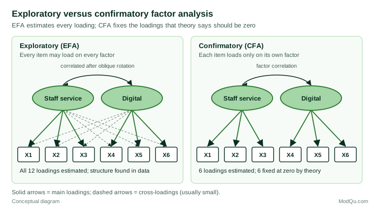
There are two main branches. Exploratory factor analysis (EFA) asks what structure the data contain, without fixing in advance which item belongs to which factor. Confirmatory factor analysis (CFA) tests a structure specified in advance by theory or by earlier research. This article explains both, works through an example, and sets out practical guidance for survey and business data.
The common factor model
Charles Spearman (1904) noticed that children's marks in different school subjects were all positively correlated, and proposed that a single general factor accounted for the pattern. Thurstone (1947) generalised the idea to several factors and introduced the principle of simple structure, in which each variable relates mainly to one factor. The modern common factor model writes each standardised item as:
xi = λi1F1 + λi2F2 + … + λimFm + ui
The F terms are the common factors shared by several items, the λ terms are factor loadings, and ui is the unique part of the item, which combines measurement error with anything specific to that question. An item's communality is the share of its variance explained by the common factors; the rest is its uniqueness. The model implies that items correlate with each other only because they share common factors.
Factor analysis is not principal component analysis
Principal component analysis (PCA), which goes back to Pearson (1901), is often run in the same software menus and is frequently confused with factor analysis. PCA builds weighted sums of the observed variables that capture as much of their total variance as possible. It does not separate shared variance from unique variance and does not model a latent cause. Factor analysis models only the shared variance. When items have modest communalities, as rating questions often do, the two methods can give noticeably different results: Widaman (1993) showed that component loadings tend to overstate the loadings of the underlying factors. PCA is a sound tool for data reduction; factor analysis is the right tool when the goal is to understand or measure latent constructs (Fabrigar et al., 1999).
Exploratory factor analysis step by step
1. Check that the data are suitable
Factor analysis needs items that are correlated with one another. The Kaiser–Meyer–Olkin measure of sampling adequacy summarises how much of the correlation among items is shared rather than specific to pairs of items. Kaiser (1974) described values in the 0.90s as "marvelous" and those below 0.50 as "unacceptable". Items that correlate weakly with everything else are unlikely to define a factor.
Sample size matters, but simple rules such as "ten respondents per item" are unreliable. MacCallum et al. (1999) showed that the sample needed depends mostly on the communalities and on how many items measure each factor. With high communalities and several strong items per factor, samples of around 100 can recover the structure well; with low communalities and few items per factor, much larger samples are needed.
2. Decide how many factors to extract
This is the most consequential decision in EFA. Extracting too few factors merges distinct dimensions; extracting too many splits real ones and creates factors that do not replicate. Several rules are in common use:
- Eigenvalues greater than one. The rule popularised by Kaiser (1960) keeps every factor whose eigenvalue exceeds 1. It is the default in many programs, but in a comparison of five rules by Zwick and Velicer (1986) it consistently overestimated the number of factors.
- The scree test. Cattell (1966) suggested plotting the eigenvalues in descending order and keeping the factors before the point where the curve levels off. It is useful but subjective.
- Parallel analysis. Horn (1965) proposed comparing the observed eigenvalues with those from random data sets of the same size. Only factors whose eigenvalues exceed those expected from random noise are retained.
- The minimum average partial test. Velicer (1976) proposed extracting factors until the average squared partial correlation among the items stops falling.
Zwick and Velicer (1986) found parallel analysis and the minimum average partial test to be the most accurate. Good practice is to use them as the main guide and to compare solutions with one factor more and one fewer, choosing the one that is most interpretable (Fabrigar et al., 1999).
3. Choose an estimation method
Maximum likelihood estimation provides standard errors and fit statistics but assumes approximately normal data. Principal axis factoring makes fewer distributional assumptions and is robust when the data are clearly non-normal. Both estimate common factors; neither is the same as PCA.
4. Rotate the solution
The initial solution is mathematically valid but hard to interpret, so the factors are rotated towards simple structure. Orthogonal rotations such as varimax (Kaiser, 1958) keep the factors uncorrelated. Oblique rotations such as oblimin and promax allow them to correlate. In survey research, constructs such as staff service and value for money are almost always correlated in reality, so an oblique rotation is the more realistic default; if the factors turn out to be uncorrelated, an oblique rotation will show that too (Browne, 2001; Fabrigar et al., 1999). After an oblique rotation, interpret the pattern matrix, which shows each item's unique relationship with each factor.
5. Interpret and name the factors
Factors are named by reading the items that load strongly on them. Loadings of about 0.40 or more are often treated as meaningful, although the threshold is a convention rather than a rule. Items with no substantial loading, or with similar loadings on two factors, deserve a closer look: they may be poorly worded, ambiguous or measuring two things at once.
A worked example
A hypothetical retail bank surveys 800 customers with twelve agreement items on a seven-point scale. The analyst splits the sample at random into two halves of 400: the first for exploration, the second for confirmation.
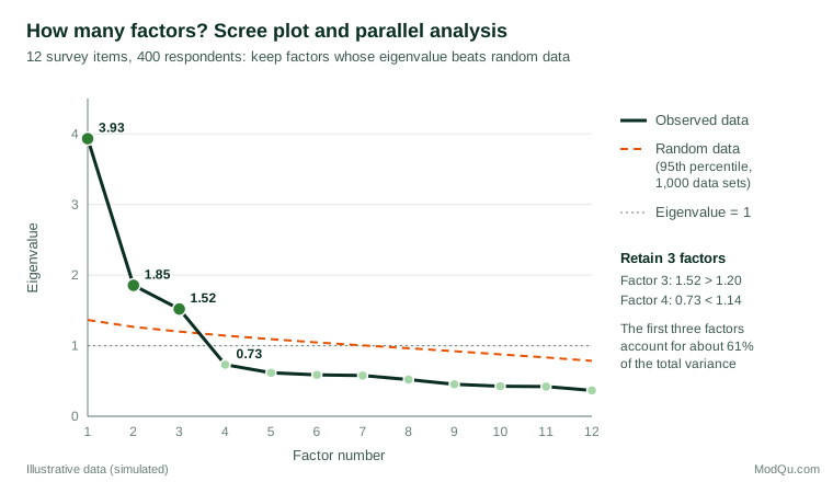
In the exploration half, the first three eigenvalues of the correlation matrix are 3.93, 1.85 and 1.52, and the fourth is 0.73. Parallel analysis with 1,000 random data sets gives 95th-percentile eigenvalues of 1.36, 1.27, 1.20 and 1.14 for the first four positions. The first three observed eigenvalues beat their random counterparts and the fourth does not, so three factors are retained. Here the eigenvalue-greater-than-one rule happens to agree, but with longer batteries it often does not.
A three-factor maximum likelihood solution with oblimin rotation gives the illustrative pattern loadings below (loadings under 0.20 are left blank for readability).
| Item (abbreviated) | Staff service | Digital experience | Value for money |
|---|---|---|---|
| Staff are courteous | 0.77 | ||
| Staff understand my needs | 0.71 | ||
| Problems are resolved quickly in branch | 0.69 | ||
| Advisers explain products clearly | 0.61 | ||
| The app is easy to use | 0.79 | ||
| Online banking is reliable | 0.70 | ||
| I can find what I need online | 0.67 | ||
| I can reach a person easily through the app | 0.31 | 0.56 | |
| Fees are fair | 0.75 | ||
| Interest rates are competitive | 0.68 | ||
| I get good value overall | 0.62 | ||
| Charges are clearly explained | 0.54 |
The factors are easy to name. The factor correlations are moderate (about 0.25 to 0.35), which supports the choice of an oblique rotation. One item, about reaching a person through the app, loads mainly on digital experience but also on staff service. This makes sense: the question mixes a digital channel with human contact. The analyst might reword it in the next wave.
Confirmatory factor analysis
In CFA the analyst specifies in advance how many factors there are, which items load on which factor, and which loadings are fixed at zero. Jöreskog (1969) developed the maximum likelihood approach that made this possible and allowed formal tests of how well the specified structure reproduces the observed correlations. CFA is also the measurement part of a full structural equation model.
Fitting and evaluating a CFA
Returning to the example, the analyst fits the three-factor structure to the second half of the sample, with each item loading only on its intended factor. The model has 78 distinct variances and covariances and 27 free parameters, leaving 51 degrees of freedom. The illustrative fit is χ²(51) = 98.4, p < 0.001; CFI = 0.972; RMSEA = 0.048; SRMR = 0.039. As with any covariance structure model, the chi-square test is very sensitive in large samples, so approximate fit indices are read alongside it. Hu and Bentler (1999) suggested values close to 0.95 or above for the CFI, close to 0.06 or below for the RMSEA and close to 0.08 or below for the SRMR, while cautioning that no single cut-off suits every model.
The fit is acceptable, and the largest residual involves the "reach a person" item, as the EFA suggested. Freeing that one cross-loading improves fit to χ²(50) = 71.6, RMSEA = 0.033. Because the change was predicted from item content and the first half of the data, it is defensible; but any change made after seeing CFA results is exploratory and should be confirmed on new data (Brown, 2015).
Reliability from the factor model
Once a factor structure is confirmed, the loadings give a direct estimate of how reliably each scale measures its construct. Cronbach's alpha (Cronbach, 1951) is the most widely reported index, but it assumes that all items load equally on the factor. McNeish (2018) reviews why this assumption rarely holds and recommends coefficients such as omega, computed from the CFA loadings. For the staff service factor, with standardised loadings of 0.77, 0.71, 0.69 and 0.61 in the illustrative EFA, omega is about 0.79.
Using the results
Once the structure is settled, most projects need a score for each respondent on each factor. There are two common options. Summed or averaged scale scores add up the items assigned to each factor. They are simple, transparent and easy to reproduce in the next survey wave, which is why tracking studies usually prefer them. Factor scores weight each item by its relationship with the factor, so stronger items count for more. They make fuller use of the model but depend on the particular sample and estimation method, and different scoring methods give slightly different results. Either way, the scores still contain measurement error, which a full structural equation model can take into account.
Factor scores have several practical uses in business analysis. In driver analysis, replacing twenty correlated attributes with a few factors reduces the multicollinearity that makes individual regression coefficients unstable. In segmentation, clustering respondents on a few factor scores rather than many raw items gives segments that are easier to describe and less dominated by whichever topic had the most questions. In reporting, a handful of well-measured dimensions is easier for managers to follow than a long list of item averages.
EFA or CFA?
The choice follows the state of knowledge, not the software available.
| Situation | Better choice |
|---|---|
| New questionnaire, no established structure | EFA |
| Adapting a scale to a new market or language | EFA, then CFA on new data |
| Established scale, checking it still works | CFA |
| Comparing groups, countries or survey modes | Multi-group CFA |
| Building a full model of relationships between constructs | CFA, then a structural model |
A sound scale development project usually uses both: EFA on one sample to discover and refine the structure, and CFA on a separate sample to test it. Running EFA and CFA on the same data and reporting the CFA as confirmation is circular, because the structure was chosen to fit those data.
Comparing groups: measurement invariance
Before comparing factor means across segments, regions or languages, CFA can test whether the items work in the same way in each group. Vandenberg and Lance (2000) review the sequence of tests: the same pattern of loadings (configural invariance), equal loadings (metric invariance) and equal item intercepts (scalar invariance). Without at least scalar invariance, a difference in average scores may reflect how a translated question was understood rather than a real difference between customers.
Practical guidance for survey and business data
- Write items with the factors in mind. Factor analysis can only find dimensions that the questionnaire measures. Aim for at least three or four clearly worded items per expected factor.
- Treat rating scales as ordinal where needed. With few response categories or strongly skewed answers, Pearson correlations understate the relationships between items. Flora and Curran (2004) found that CFA based on polychoric correlations with robust weighted least squares estimation performed well for ordinal data.
- Watch for method factors. Negatively worded items, or items that share an unusual format, can form their own factor that reflects response style rather than content.
- Report enough for others to judge. State the extraction method, the rule used for the number of factors, the rotation, the full pattern matrix, factor correlations and, for CFA, the fit indices and any modifications.
Common mistakes
- Running PCA with the default settings and calling it factor analysis. Preacher and MacCallum (2003) showed how the common default combination of principal components, the eigenvalue-greater-than-one rule and varimax rotation can lead to the wrong number of factors and a distorted structure. Fabrigar et al. (1999) found such choices to be common in published research.
- Relying on the eigenvalue-greater-than-one rule. It tends to retain too many factors (Zwick & Velicer, 1986).
- Forcing factors to be uncorrelated. Varimax rotation imposes independence that most business constructs do not have.
- Treating the factor solution as fixed truth. Factor structures can vary across samples, markets and time. Confirm important structures on new data.
- Over-reading a single strong first factor. A large first eigenvalue may reflect a general halo effect or acquiescence rather than one substantive dimension.
Key takeaways
Factor analysis turns a block of correlated survey questions into a small number of interpretable dimensions. Exploratory factor analysis discovers that structure, and its key decisions are the number of factors, the estimation method and the rotation; parallel analysis and an oblique rotation are sound defaults. Confirmatory factor analysis tests a structure stated in advance, provides fit statistics and reliability estimates, and supports fair comparisons between groups. Used together, on separate samples, they give business decision-makers scales they can trust.
References
Browne, M. W. (2001). An overview of analytic rotation in exploratory factor analysis. Multivariate Behavioral Research, 36(1), 111–150. https://doi.org/10.1207/S15327906MBR3601_05
Brown, T. A. (2015). Confirmatory factor analysis for applied research (2nd ed.). Guilford Press.
Cattell, R. B. (1966). The scree test for the number of factors. Multivariate Behavioral Research, 1(2), 245–276. https://doi.org/10.1207/s15327906mbr0102_10
Cronbach, L. J. (1951). Coefficient alpha and the internal structure of tests. Psychometrika, 16(3), 297–334. https://doi.org/10.1007/BF02310555
Fabrigar, L. R., Wegener, D. T., MacCallum, R. C., & Strahan, E. J. (1999). Evaluating the use of exploratory factor analysis in psychological research. Psychological Methods, 4(3), 272–299. https://doi.org/10.1037/1082-989X.4.3.272
Flora, D. B., & Curran, P. J. (2004). An empirical evaluation of alternative methods of estimation for confirmatory factor analysis with ordinal data. Psychological Methods, 9(4), 466–491. https://doi.org/10.1037/1082-989X.9.4.466
Horn, J. L. (1965). A rationale and test for the number of factors in factor analysis. Psychometrika, 30(2), 179–185. https://doi.org/10.1007/BF02289447
Hu, L., & Bentler, P. M. (1999). Cutoff criteria for fit indexes in covariance structure analysis: Conventional criteria versus new alternatives. Structural Equation Modeling: A Multidisciplinary Journal, 6(1), 1–55. https://doi.org/10.1080/10705519909540118
Jöreskog, K. G. (1969). A general approach to confirmatory maximum likelihood factor analysis. Psychometrika, 34(2), 183–202. https://doi.org/10.1007/BF02289343
Kaiser, H. F. (1958). The varimax criterion for analytic rotation in factor analysis. Psychometrika, 23(3), 187–200. https://doi.org/10.1007/BF02289233
Kaiser, H. F. (1960). The application of electronic computers to factor analysis. Educational and Psychological Measurement, 20(1), 141–151. https://doi.org/10.1177/001316446002000116
Kaiser, H. F. (1974). An index of factorial simplicity. Psychometrika, 39(1), 31–36. https://doi.org/10.1007/BF02291575
MacCallum, R. C., Widaman, K. F., Zhang, S., & Hong, S. (1999). Sample size in factor analysis. Psychological Methods, 4(1), 84–99. https://doi.org/10.1037/1082-989X.4.1.84
McNeish, D. (2018). Thanks coefficient alpha, we'll take it from here. Psychological Methods, 23(3), 412–433. https://doi.org/10.1037/met0000144
Pearson, K. (1901). LIII. On lines and planes of closest fit to systems of points in space. The London, Edinburgh, and Dublin Philosophical Magazine and Journal of Science, 2(11), 559–572. https://doi.org/10.1080/14786440109462720
Preacher, K. J., & MacCallum, R. C. (2003). Repairing Tom Swift's electric factor analysis machine. Understanding Statistics, 2(1), 13–43. https://doi.org/10.1207/S15328031US0201_02
Spearman, C. (1904). "General intelligence," objectively determined and measured. The American Journal of Psychology, 15(2), 201–292. https://doi.org/10.2307/1412107
Thurstone, L. L. (1947). Multiple-factor analysis: A development and expansion of The vectors of mind. University of Chicago Press.
Vandenberg, R. J., & Lance, C. E. (2000). A review and synthesis of the measurement invariance literature: Suggestions, practices, and recommendations for organizational research. Organizational Research Methods, 3(1), 4–70. https://doi.org/10.1177/109442810031002
Velicer, W. F. (1976). Determining the number of components from the matrix of partial correlations. Psychometrika, 41(3), 321–327. https://doi.org/10.1007/BF02293557
Widaman, K. F. (1993). Common factor analysis versus principal component analysis: Differential bias in representing model parameters? Multivariate Behavioral Research, 28(3), 263–311. https://doi.org/10.1207/s15327906mbr2803_1
Zwick, W. R., & Velicer, W. F. (1986). Comparison of five rules for determining the number of components to retain. Psychological Bulletin, 99(3), 432–442. https://doi.org/10.1037/0033-2909.99.3.432