
Statistics · Tests and models
Cluster Analysis for Market Segmentation
How cluster analysis groups customers into segments from survey data, how k-means and hierarchical methods work, how to choose the number of segments, and how to judge whether they are real and useful.
Few customer bases are uniform. Some buyers chase the lowest price, some pay for quality, and some barely think about the category at all. Treating everyone the same wastes money on people who will never respond and underserves the people who would. Wendell Smith (1956) gave this idea its modern name, market segmentation: dividing a heterogeneous market into smaller groups whose needs are more alike, so that products, prices and messages can be fitted to each.
Segments can be defined in advance from a single known variable, such as age band or region. This is often called a priori or commonsense segmentation. Much of the value of survey research, however, lies in finding segments that nobody specified in advance: groups of respondents who share a pattern of attitudes, needs or behaviours across many questions at once. The family of methods used to find such groups is cluster analysis. This article explains how the main methods work, walks through a worked example, and sets out the decisions and checks that separate a defensible segmentation from an arbitrary one.
What cluster analysis does
Cluster analysis sorts cases into groups so that cases in the same group are similar to one another and different from cases in other groups. Unlike regression or classification, there is no outcome variable to predict and no "correct" answer to check against. The method is exploratory: it proposes a grouping, and the analyst must decide whether that grouping is stable, interpretable and useful (Everitt et al., 2011).
That lack of ground truth is the central fact to keep in mind. A clustering algorithm will always return clusters, even when the data contain no natural groups at all. Jain (2010) puts it plainly in his review of fifty years of clustering research: there is no single best algorithm, and the notion of a "cluster" depends on the data and the purpose. A segmentation is therefore a modelling decision, not a discovery that the software simply reports.
In market research, the inputs (sometimes called segmentation bases) are usually attitude ratings, stated needs, benefits sought, purchase behaviour or a mix of these. Descriptor variables such as age, income and media use are typically kept out of the clustering itself and used afterwards to profile the segments and work out how to reach them (Wedel & Kamakura, 2000). Punj and Stewart (1983), in an early and still useful review for the Journal of Marketing Research, stressed that the choice of variables shapes the result more than the choice of algorithm.
Measuring similarity
Every clustering method needs a way to say how alike two respondents are. For numeric ratings, the usual choice is Euclidean distance, the straight-line distance between two respondents' score profiles:
d(i, j) = √[(xi1 − xj1)2 + (xi2 − xj2)2 + … + (xip − xjp)2]
Here xik is respondent i's score on variable k, and there are p variables. Two practical points follow from the formula. First, variables measured on larger scales dominate the distance. A spending variable measured in dollars will swamp a five-point rating unless the variables are put on comparable scales. Milligan and Cooper (1988) compared several ways of standardising variables before clustering and found that the choice matters, with division by the range performing well in their simulations; dividing by the standard deviation (z-scores) is also common. Second, every variable counts equally unless it is weighted. Including ten questions about price and two about service implicitly makes price five times as important.
Survey data often mix numeric, ordinal and categorical variables. Gower's (1971) general similarity coefficient handles such mixtures by computing a suitable similarity for each variable and averaging them, and it is the usual starting point for clustering mixed data with hierarchical or medoid-based methods (Kaufman & Rousseeuw, 1990).
The main families of methods
Hierarchical clustering
Agglomerative hierarchical methods start with every respondent as a separate cluster and repeatedly merge the two closest clusters until only one remains. The result is a tree, or dendrogram, that can be cut at any height to give a chosen number of groups. Methods differ in how they define the distance between two clusters. Single linkage uses the closest pair of members and tends to produce long, straggling chains; complete linkage uses the farthest pair; average linkage uses the mean of all pairwise distances. Ward's method merges the pair of clusters whose union causes the smallest increase in total within-cluster sum of squares (Ward, 1963). Because it favours compact groups of similar size, Ward's method is widely used for segmentation.
Hierarchical methods are transparent and do not require the number of clusters in advance, but they have two weaknesses. Merges cannot be undone, so an early poor merge carries through to the final solution, and the full distance matrix becomes expensive for very large samples.
K-means
K-means clustering is the workhorse of applied segmentation. The analyst chooses the number of clusters, k. The algorithm places k starting centres, assigns each respondent to the nearest centre, recomputes each centre as the mean of its members, and repeats until assignments stop changing. The procedure is usually credited to MacQueen (1967), who named it, and to Lloyd (1982), whose algorithm from a 1957 technical report was published decades later. Steinley (2006) gives a thorough synthesis of its history and properties.
K-means minimises the within-cluster sum of squares:
W = Σc=1…k Σi in c ‖xi − mc‖2
where mc is the centre (mean profile) of cluster c. The algorithm is fast and scales to very large files, but it finds a local rather than a guaranteed global minimum. Different random starts can give different answers, so good practice is to run it many times from different starting points and keep the solution with the smallest W (Steinley, 2006). K-means also prefers roughly spherical clusters of similar spread, and because it uses means it is sensitive to outliers. A common hybrid uses Ward's method to find starting centres and k-means to refine them, an approach recommended by Punj and Stewart (1983).
Partitioning around medoids
Kaufman and Rousseeuw (1990) proposed partitioning around medoids (PAM), which uses actual respondents, called medoids, as cluster centres instead of averages. It works with any dissimilarity, including Gower's coefficient, and is less affected by extreme cases than k-means. Each segment is then represented by a real, typical respondent, which some clients find easier to understand than an abstract average profile.
Model-based clustering and latent class analysis
Model-based methods treat the data as a mixture of probability distributions, one per segment, and estimate each respondent's probability of belonging to each segment. Fraley and Raftery (2002) describe Gaussian mixture models for numeric data, usually fitted with the expectation–maximisation (EM) algorithm, which alternates between estimating membership probabilities and updating each segment's parameters. The same idea applied to categorical survey answers is latent class analysis. Mixture models give a formal basis for choosing the number of segments through likelihood-based criteria such as the Bayesian information criterion (BIC) (Schwarz, 1978), and they allow clusters with different shapes and sizes. Wedel and Kamakura (2000) argue that mixture models are the most statistically principled route to segmentation, although they demand more care in estimation and larger samples than k-means.
A worked example
Suppose a hypothetical online retailer surveys 800 customers. Two composite scores, each the average of several rating items on a 0 to 10 scale, summarise price sensitivity and interest in premium features. Both scores are standardised and k-means is run for every value of k from 1 to 8, with 25 random starts each. The numbers below come from simulated, illustrative data.
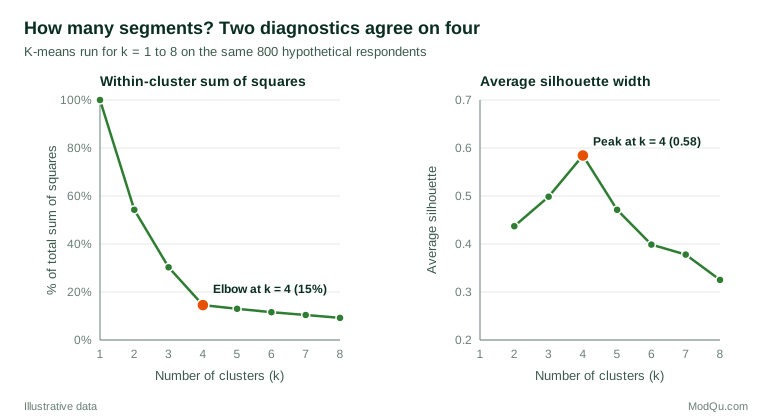
Figure 1 shows two common diagnostics. The left panel tracks the within-cluster sum of squares as a share of the total. Adding clusters always reduces it, so the question is where the gains flatten out. Here the share falls from 100% to 54%, 30% and then 15% at four clusters, after which each extra cluster removes only one or two more percentage points. This bend is called the "elbow". The right panel shows the average silhouette width (Rousseeuw, 1987), which compares, for each respondent, the average distance to members of their own cluster (a) with the average distance to the nearest other cluster (b):
s(i) = (b(i) − a(i)) ÷ max{a(i), b(i)}
Values near 1 mean a respondent sits comfortably inside their cluster; values near 0 mean they lie on a boundary; negative values suggest they may be in the wrong cluster. The average silhouette here peaks at 0.58 for four clusters. Kaufman and Rousseeuw (1990) suggest that an average above about 0.5 indicates a reasonable structure and above 0.7 a strong one, so this solution is reasonable rather than overwhelming.
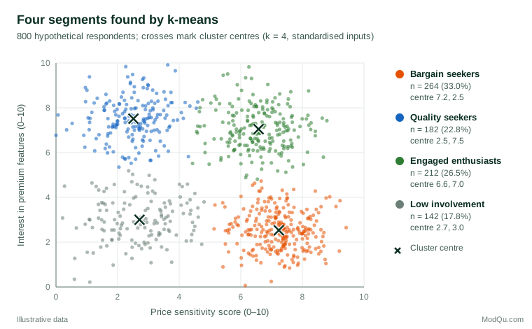
Figure 2 shows the resulting segments. The largest group, about a third of the sample, combines high price sensitivity with little interest in premium features, a natural target for value ranges and promotions. A second group (23%) shows the opposite pattern, and a third (27%) scores highly on both, suggesting customers who want premium features but watch the price, perhaps responsive to bundles or loyalty rewards. The smallest group (18%) is low on both, which may indicate low involvement in the category, or simply respondents who gave little thought to the questions. Names such as "bargain seekers" are the analyst's labels, chosen after inspecting the centres; they are not produced by the algorithm.
Two further checks support the solution. Re-running k-means on 100 bootstrap resamples and comparing each result with the original using the adjusted Rand index (Hubert & Arabie, 1985), which equals 1 for identical partitions and about 0 for chance agreement, gave a median of 0.99. The segments are therefore highly stable in this illustrative case. In practice, the next step would be to profile the segments on descriptor variables, such as age, channel use and spending, and to test whether they differ in ways that matter for decisions.
Real survey data are rarely this tidy. The example uses two variables and well-separated groups so that the logic is easy to follow on a single page. With ten or twenty attitude items, clusters usually overlap far more, average silhouettes in the weak range below 0.5 are typical, and the diagnostics may point to different numbers of segments. Each of these situations calls for more judgement, not less.
Choosing the number of segments
There is no single correct method for choosing k. In a classic simulation study, Milligan and Cooper (1985) compared 30 stopping rules on data with known structure and found large differences in performance. The Calinski–Harabasz index, the ratio of between-cluster to within-cluster variation adjusted for the number of clusters (Caliński & Harabasz, 1974), was among the best performers. The gap statistic of Tibshirani et al. (2001) compares the observed within-cluster dispersion with what would be expected from data with no cluster structure, and it has the useful property of being able to suggest that a single cluster (no segmentation) is the best description. For mixture models, BIC is the usual criterion (Fraley & Raftery, 2002).
Statistical indices should inform the choice, not make it. Dolnicar et al. (2018) emphasise that a segmentation must also be usable: each segment needs to be large enough to justify a separate strategy, distinct enough to respond differently, reachable through identifiable channels, and stable over time. A seven-segment solution that fits slightly better than a four-segment one may still be the wrong choice if the marketing team can act on only three or four groups. A sensible approach is to examine two or three candidate solutions side by side, compare their stability and interpretability, and agree the final choice with the people who will use it.
Are the segments real?
Because clustering always produces an answer, validation is the most important stage and the most often skipped. Several complementary checks are available.
- Stability. Re-run the analysis on bootstrap samples or random halves of the data and measure agreement with the adjusted Rand index. Hennig (2007) proposed assessing stability cluster by cluster, since one solid segment may coexist with another that dissolves under resampling.
- Sensitivity to method. Compare k-means, Ward's method and a mixture model. Segments that appear under several methods deserve more confidence than those produced by one algorithm and one set of starting values.
- Meaningful external differences. Segments should differ on variables not used to form them, such as purchase frequency, retention or response to a past campaign. This is the strongest evidence that they matter commercially.
- Replication. Where possible, check whether a similar structure appears in a fresh sample or a later wave of the same tracker.
Dolnicar et al. (2018) make a further point that is often overlooked. Many consumer data sets do not contain natural, well-separated clusters at all. In that case, clustering still produces a useful partition of a continuous market, but the analyst should describe it as constructed segmentation rather than claim to have revealed hidden types of customer. Being honest about which case applies protects the client from over-interpreting boundaries that are partly arbitrary.
Practical guidance for survey and market research data
Choose segmentation variables with care. Select variables that relate to the business decision at hand. Avoid large blocks of near-duplicate items, which silently give one theme extra weight. Hastie et al. (2009) note that, in unsupervised learning, the choice of variables and dissimilarity largely determines what structure is found.
Watch for response styles. Some respondents tend to agree with everything or to use only the extremes of a scale. Baumgartner and Steenkamp (2001) showed that such response styles distort scale scores and the relationships between them in marketing surveys. When clustering raw ratings, response styles can create a "yea-saying" segment that reflects how people answer questions rather than what they think. Within-respondent centring or item formats that are less prone to acquiescence can help.
Screen out careless responses. Respondents who speed through a questionnaire or give the same answer to every item form spurious clusters of their own. Meade and Craig (2012) review methods for detecting careless responding, including response time, long strings of identical answers and consistency checks, and these should be applied before clustering.
Be cautious with factor-cluster segmentation. A common practice is to reduce many items with factor analysis or principal component analysis and then cluster the component scores. Dolnicar and Grün (2008) showed in simulations that this "factor-cluster" approach can hide segment structure that clustering on the original items would recover, because the reduction step discards information that distinguishes the groups. Reduce variables only for a clear reason, and compare the result with clustering on a well-chosen subset of the original items.
Handle outliers and small clusters. A few extreme respondents can pull a k-means centre or form a tiny cluster of their own. Medoid-based methods, robust scaling or trimming can reduce their influence (Kaufman & Rousseeuw, 1990). It is worth inspecting very small clusters individually: they sometimes reveal a genuine niche, such as a handful of high-value business buyers in a consumer sample, but more often they contain data errors or careless respondents.
Plan for assigning new customers. A segmentation is only useful if new customers can be placed in a segment. Short "golden question" scoring tools or classification models trained on the segment labels allow segments to be applied in a customer database or future survey.
Mind the sample. Segment sizes estimated from a weighted survey should use the survey weights, and small segments come with wide margins of error. A segment that makes up 5% of a 400-person sample contains about 20 respondents, too few for confident profiling.
Common mistakes
- Treating clusters as natural kinds. The algorithm partitions the data whatever their structure. Segments are useful summaries, not proof that customers come in discrete types.
- Reporting a single run. K-means with one random start, or a single algorithm without stability checks, can produce a solution that would not reappear on another day.
- Ignoring scale. Clustering unstandardised variables measured on different scales lets the variable with the largest spread decide the segments.
- Clustering on everything available. Adding irrelevant variables dilutes real structure and makes segments harder to interpret.
- Testing segment differences on the clustering variables. Segments formed to differ on certain variables will, by construction, differ significantly on those variables. Significance tests on the inputs are therefore meaningless; only differences on external variables are informative.
- Letting labels outrun the evidence. Vivid segment names and personas are helpful for communication, but they can make modest differences sound like sharp divides. Report segment centres and overlap alongside the labels.
Key takeaways
Cluster analysis turns many survey answers into a small number of customer groups that can guide product, pricing and communication decisions. K-means, Ward's hierarchical method, medoid-based methods and mixture models each have strengths, and the choice of variables, scaling and dissimilarity often matters more than the algorithm. Because every method returns clusters whether or not they exist, the number of segments should be chosen using several diagnostics together with business judgement, and the result should be checked for stability, robustness across methods, and meaningful differences on outside variables. A well-validated segmentation, described honestly as either natural or constructed, is a durable asset; an unvalidated one is a set of labels on noise.
References
Baumgartner, H., & Steenkamp, J.-B. E. M. (2001). Response styles in marketing research: A cross-national investigation. Journal of Marketing Research, 38(2), 143–156. https://doi.org/10.1509/jmkr.38.2.143.18840
Caliński, T., & Harabasz, J. (1974). A dendrite method for cluster analysis. Communications in Statistics, 3(1), 1–27. https://doi.org/10.1080/03610927408827101
Dolnicar, S., & Grün, B. (2008). Challenging "factor–cluster segmentation". Journal of Travel Research, 47(1), 63–71. https://doi.org/10.1177/0047287508318910
Dolnicar, S., Grün, B., & Leisch, F. (2018). Market segmentation analysis: Understanding it, doing it, and making it useful. Springer. https://doi.org/10.1007/978-981-10-8818-6
Everitt, B. S., Landau, S., Leese, M., & Stahl, D. (2011). Cluster analysis (5th ed.). Wiley. https://doi.org/10.1002/9780470977811
Fraley, C., & Raftery, A. E. (2002). Model-based clustering, discriminant analysis, and density estimation. Journal of the American Statistical Association, 97(458), 611–631. https://doi.org/10.1198/016214502760047131
Gower, J. C. (1971). A general coefficient of similarity and some of its properties. Biometrics, 27(4), 857–871. https://doi.org/10.2307/2528823
Hastie, T., Tibshirani, R., & Friedman, J. (2009). The elements of statistical learning: Data mining, inference, and prediction (2nd ed.). Springer. https://doi.org/10.1007/978-0-387-84858-7
Hennig, C. (2007). Cluster-wise assessment of cluster stability. Computational Statistics & Data Analysis, 52(1), 258–271. https://doi.org/10.1016/j.csda.2006.11.025
Hubert, L., & Arabie, P. (1985). Comparing partitions. Journal of Classification, 2(1), 193–218. https://doi.org/10.1007/BF01908075
Jain, A. K. (2010). Data clustering: 50 years beyond K-means. Pattern Recognition Letters, 31(8), 651–666. https://doi.org/10.1016/j.patrec.2009.09.011
Kaufman, L., & Rousseeuw, P. J. (1990). Finding groups in data: An introduction to cluster analysis. Wiley. https://doi.org/10.1002/9780470316801
Lloyd, S. (1982). Least squares quantization in PCM. IEEE Transactions on Information Theory, 28(2), 129–137. https://doi.org/10.1109/TIT.1982.1056489
MacQueen, J. (1967). Some methods for classification and analysis of multivariate observations. In L. M. Le Cam & J. Neyman (Eds.), Proceedings of the Fifth Berkeley Symposium on Mathematical Statistics and Probability (Vol. 1, pp. 281–297). University of California Press.
Meade, A. W., & Craig, S. B. (2012). Identifying careless responses in survey data. Psychological Methods, 17(3), 437–455. https://doi.org/10.1037/a0028085
Milligan, G. W., & Cooper, M. C. (1985). An examination of procedures for determining the number of clusters in a data set. Psychometrika, 50(2), 159–179. https://doi.org/10.1007/BF02294245
Milligan, G. W., & Cooper, M. C. (1988). A study of standardization of variables in cluster analysis. Journal of Classification, 5(2), 181–204. https://doi.org/10.1007/BF01897163
Punj, G., & Stewart, D. W. (1983). Cluster analysis in marketing research: Review and suggestions for application. Journal of Marketing Research, 20(2), 134–148. https://doi.org/10.1177/002224378302000204
Rousseeuw, P. J. (1987). Silhouettes: A graphical aid to the interpretation and validation of cluster analysis. Journal of Computational and Applied Mathematics, 20, 53–65. https://doi.org/10.1016/0377-0427(87)90125-7
Schwarz, G. (1978). Estimating the dimension of a model. The Annals of Statistics, 6(2), 461–464. https://doi.org/10.1214/aos/1176344136
Smith, W. R. (1956). Product differentiation and market segmentation as alternative marketing strategies. Journal of Marketing, 21(1), 3–8. https://doi.org/10.1177/002224295602100102
Steinley, D. (2006). K-means clustering: A half-century synthesis. British Journal of Mathematical and Statistical Psychology, 59(1), 1–34. https://doi.org/10.1348/000711005X48266
Tibshirani, R., Walther, G., & Hastie, T. (2001). Estimating the number of clusters in a data set via the gap statistic. Journal of the Royal Statistical Society Series B: Statistical Methodology, 63(2), 411–423. https://doi.org/10.1111/1467-9868.00293
Ward, J. H., Jr. (1963). Hierarchical grouping to optimize an objective function. Journal of the American Statistical Association, 58(301), 236–244. https://doi.org/10.1080/01621459.1963.10500845
Wedel, M., & Kamakura, W. A. (2000). Market segmentation: Conceptual and methodological foundations (2nd ed.). Springer. https://doi.org/10.1007/978-1-4615-4651-1