
Statistics · Communication and misuse
Statistical Process Control and Monitoring for Ongoing Knowledge Quality
How Shewhart control charts separate routine variation from real problems, how to build and read a p-chart, and how to monitor recurring surveys, data pipelines and business metrics without overreacting.
Much of the information organisations rely on is produced again and again: weekly trackers, monthly customer satisfaction scores, daily data feeds and dashboards. The quality of each new figure depends on a process that can drift, break or change without anyone noticing. Statistical process control (SPC) offers a simple discipline for watching such processes. It was developed by Walter Shewhart at Bell Telephone Laboratories in the 1920s for manufacturing (Shewhart, 1931), but its logic applies equally to any repeated measurement, including the production of statistics themselves.
Common causes and special causes
Shewhart's key insight was that every process varies, and that the variation comes from two kinds of source. Common-cause variation is the background noise built into a stable process: many small influences that no one can single out. Special-cause variation comes from something specific and identifiable, such as a broken questionnaire route, a new supplier or a coding change. A process showing only common-cause variation is said to be in statistical control, which means its future behaviour can be predicted within limits.
The distinction matters because the two call for different responses. Special causes should be investigated and removed. Common-cause variation can only be reduced by changing the process itself. Reacting to every rise and fall as if it had a special cause, often called tampering, usually makes a process worse rather than better (Deming, 1975; Wheeler, 2000). Deming (1953) also stressed that monitoring a process is an analytic problem, concerned with predicting what the process will do next, rather than an enumerative one about a fixed population.
Anatomy of a Shewhart control chart
A control chart plots a statistic over time against three horizontal lines: a centre line at the process average and upper and lower control limits, usually set three standard errors either side. If the process is stable and the statistic is roughly normal, only about 0.27% of points will fall outside three-sigma limits by chance, which is about one false alarm in 370 points (Montgomery, 2020).
The right chart depends on the data:
| Data type | Chart | Typical use |
|---|---|---|
| Single measurements | Individuals and moving range (XmR) | Daily revenue, one score per week |
| Means of small subgroups | X̄ and R or X̄ and S | Average of several readings per period |
| Proportions | p-chart (np-chart if n is fixed) | Share of interviews flagged, response rate |
| Counts of events | c-chart or u-chart | Complaints, data-entry errors per batch |
Practitioners distinguish two phases (Woodall, 2000). In Phase I, historical data are used to check whether the process was stable and to estimate the centre line and limits, after removing periods with known special causes. In Phase II, those fixed limits are used to monitor new data as they arrive. Woodall (2000) argues that much confusion about control charts comes from mixing up these two purposes.
Rules for signals
The basic signal is a point beyond a control limit. To detect smaller or gradual shifts, supplementary run rules were added, such as eight points in a row on one side of the centre line, or two of three consecutive points beyond two sigma (Western Electric Company, 1956). Each extra rule increases sensitivity but also raises the false alarm rate, so teams should choose a small set in advance. Shewhart charts are good at catching large, sudden changes and relatively slow to detect small persistent shifts. For those, the cumulative sum (CUSUM) chart (Page, 1954) and the exponentially weighted moving average (EWMA) chart (Roberts, 1959) accumulate evidence across points and are usually more sensitive.
A worked example: a p-chart for interview quality
Consider a hypothetical online survey that runs every week. Each completed interview passes automated quality checks for speeding, straight-lining and inconsistent answers, and the team monitors the share of interviews flagged. The number of completes varies from about 300 to 700 per week, so a p-chart with limits that vary by week is appropriate:
UCLi, LCLi = p̄ ± 3 √( p̄(1 − p̄) ÷ ni )
Here p̄ is the overall flagged share in a stable baseline period and ni is the number of completes in week i. In the illustrative data, weeks 1 to 20 give p̄ = 6.0%. For a week with 500 completes the limits are about 2.8% to 9.1%; with 310 completes they widen to about 1.9% to 10.0%, because smaller samples vary more.
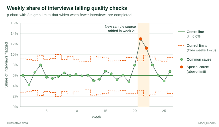
Weeks 1 to 20 stay within their limits, including week 4 at 8.0%, which might have prompted alarm if judged by eye. In week 21 the flagged share jumps to 13.0% against an upper limit of 8.8%, and week 22 remains high at 11.2%. Investigation traces both to a new sample source added in week 21. Once that source is removed, weeks 23 to 26 return to the usual range. The chart did two jobs: it prevented a false alarm in week 4 and gave a clear, early signal in week 21.
Monitoring surveys and business data
Survey organisations increasingly use paradata, such as interview timings, device type and contact attempts, to monitor fieldwork as it happens (Kreuter, 2013). Control charts turn those streams into early warnings about the components of total survey error, from coverage and nonresponse to measurement and processing (Groves & Lyberg, 2010). The same approach suits business metrics: weekly conversion rates, complaint counts, data-pipeline row counts and the share of missing values in a feed. In healthcare, SPC has become a standard tool for monitoring and improving services (Benneyan et al., 2003).
When the aim is to compare many units at one time, such as stores, regions or interviewers, rather than one process over time, a funnel plot applies the same limits idea, with limits that narrow as the unit size grows (Spiegelhalter, 2005).
Practical guidance
- Start with a stable baseline. Use at least 20 to 25 periods to set limits, and exclude periods with known special causes.
- Freeze limits in Phase II. Recalculating limits every period lets a slow drift become the new normal. Revise them only after a deliberate, documented process change.
- Match the chart to the data. Use p- or u-charts for rates with varying denominators and XmR charts for single values.
- Watch for overdispersion. With very large samples, binomial limits can become so narrow that almost every point signals, because real period-to-period variation exceeds sampling variation. Spiegelhalter (2005) shows how to widen limits to allow for this.
- Agree on responses in advance. Decide who investigates a signal, how quickly and how findings are recorded.
Common mistakes
- Confusing control limits with targets. Control limits describe what the process does; specification limits or targets describe what the business wants.
- Ignoring autocorrelation. Many business series carry seasonality or trend. Charts assume independent points, so model such patterns first or chart the residuals (Montgomery, 2020).
- Using too many rules. Every added run rule brings more false alarms.
- Treating "in control" as "good". A stable process can be stably poor; control charts show predictability, not acceptability.
Key takeaways
Shewhart control charts give a disciplined way to tell routine noise from real change in any recurring measurement. A centre line, three-sigma limits estimated from a stable baseline and a few agreed signal rules are enough to avoid both overreaction and complacency. Applied to survey fieldwork, data pipelines and business indicators, they keep the quality of ongoing knowledge visible and help teams fix the process rather than chase the numbers.
References
Benneyan, J. C., Lloyd, R. C., & Plsek, P. E. (2003). Statistical process control as a tool for research and healthcare improvement. Quality and Safety in Health Care, 12(6), 458–464. https://doi.org/10.1136/qhc.12.6.458
Deming, W. E. (1953). On the distinction between enumerative and analytic surveys. Journal of the American Statistical Association, 48(262), 244–255. https://doi.org/10.1080/01621459.1953.10483470
Deming, W. E. (1975). On probability as a basis for action. The American Statistician, 29(4), 146–152. https://doi.org/10.1080/00031305.1975.10477402
Groves, R. M., & Lyberg, L. (2010). Total survey error: Past, present, and future. Public Opinion Quarterly, 74(5), 849–879. https://doi.org/10.1093/poq/nfq065
Kreuter, F. (Ed.). (2013). Improving surveys with paradata: Analytic uses of process information. Wiley. https://doi.org/10.1002/9781118596869
Montgomery, D. C. (2020). Introduction to statistical quality control (8th ed.). Wiley.
Page, E. S. (1954). Continuous inspection schemes. Biometrika, 41(1–2), 100–115. https://doi.org/10.1093/biomet/41.1-2.100
Roberts, S. W. (1959). Control chart tests based on geometric moving averages. Technometrics, 1(3), 239–250. https://doi.org/10.1080/00401706.1959.10489860
Shewhart, W. A. (1931). Economic control of quality of manufactured product. Van Nostrand.
Spiegelhalter, D. J. (2005). Funnel plots for comparing institutional performance. Statistics in Medicine, 24(8), 1185–1202. https://doi.org/10.1002/sim.1970
Western Electric Company. (1956). Statistical quality control handbook. Western Electric Company.
Wheeler, D. J. (2000). Understanding variation: The key to managing chaos (2nd ed.). SPC Press.
Woodall, W. H. (2000). Controversies and contradictions in statistical process control. Journal of Quality Technology, 32(4), 341–350. https://doi.org/10.1080/00224065.2000.11980013