
Statistics · Communication and misuse
Data Privacy in Statistics: Disclosure Control and Differential Privacy
Why published tables and datasets can reveal individuals, how traditional disclosure control protects them, and what differential privacy adds, with a worked example and practical guidance for survey data.
Every survey and customer database rests on a promise: the information people provide will be used for statistics, not to single them out. Keeping that promise is harder than it looks. Removing names is not enough, because a combination of ordinary characteristics can be as identifying as a name, and many aggregate results released together can be pieced back into the records behind them. Statistical disclosure control is the body of methods that national statistical offices and research organisations use to release useful results while limiting that risk (Hundepool et al., 2012). Differential privacy is a newer, mathematically defined standard that has changed how the field thinks about the problem (Dwork & Roth, 2014).
How "anonymous" data reveal people
Disclosure takes two main forms. Identity disclosure happens when a record or table cell can be linked to a known person. Attribute disclosure happens when something new is learned about a person, for example when every member of a small group gave the same answer, so knowing someone belongs to the group reveals their answer.
The evidence that de-identified data can be re-identified is strong. Sweeney (2002) showed that hospital discharge records stripped of names could be matched to a public voter list using postal code, birth date and sex, and reported that this combination is probably unique for a large majority of the United States population. Narayanan and Shmatikov (2008) re-identified subscribers in a released film-rating dataset by linking a handful of ratings and approximate dates to public reviews. Rocher et al. (2019) estimated that 99.98% of Americans would be correctly re-identified in any dataset using 15 demographic attributes.
Aggregates are not automatically safe either. Dinur and Nissim (2003) proved that if too many statistics are answered too accurately, an attacker can reconstruct most of the underlying confidential records. Garfinkel et al. (2019) describe how this kind of database reconstruction attack applies to the many tables a census publishes, and why it led the United States Census Bureau to rethink its protection methods. The lesson for any data publisher is that risk depends on everything released, not on each table in isolation.
Traditional statistical disclosure control
Classical disclosure control modifies the data or outputs, guided by judgement about likely intruders and what they already know (Hundepool et al., 2012).
Tabular data. Common rules include a minimum cell size (often called a threshold rule, for example no published cell based on fewer than 5 or 10 respondents) and dominance rules for business data, where one large firm could otherwise be deduced from an industry total. Risky cells are protected by primary suppression, but totals often allow suppressed values to be recovered by subtraction, so secondary suppression of further cells is needed. Alternatives include collapsing categories and rounding.
Microdata. For record-level files, agencies remove direct identifiers and then reduce the detail of key variables: coarsening geography and age bands, top-coding incomes, swapping a small share of values between similar records, or adding noise. A formal target is k-anonymity, which requires each combination of quasi-identifiers (the variables an intruder could match on) to be shared by at least k records (Sweeney, 2002). Because a group of k people can still share the same sensitive answer, l-diversity adds the requirement that each group contains several distinct sensitive values (Machanavajjhala et al., 2007).
Synthetic data. Rubin (1993) proposed releasing artificial records drawn from a model fitted to the confidential data, so that no released row belongs to a real person while key statistical relationships are preserved. Synthetic data are only as good as the model that generated them (Drechsler, 2011).
These methods are practical, but their protection is judged against assumed attacks rather than proved, and repeated releases can undo them.
Differential privacy
Differential privacy, introduced by Dwork et al. (2006), changes the question. Instead of asking whether a particular release looks safe, it asks whether the output of an analysis would be almost the same whether or not any one person's data were included. If it would, no one can learn much about that person from the output, whatever outside information they hold.
Formally, a randomised procedure M is ε-differentially private if, for any two datasets D and D′ that differ in one person's record, and any set of possible outputs S:
P[M(D) ∈ S] ≤ eε × P[M(D′) ∈ S]
The privacy-loss parameter ε (epsilon) sets the strength of protection. Small values, such as 0.1 to 1, mean that any one person's presence changes the probability of any result very little; larger values allow more leakage in exchange for more accurate results.
The Laplace mechanism
The simplest way to achieve differential privacy is to add random noise to each statistic, scaled to how much one person can change it. This maximum change is the sensitivity, Δf. For a count, adding or removing one person changes the answer by at most 1, so Δf = 1. The Laplace mechanism releases:
released value = true value + Laplace(0, Δf ÷ ε)
Because the noise distribution is known, its size can be stated in advance: for a count with sensitivity 1, 95% of the noise falls within ±ln(20) ÷ ε, or about ±3.0 ÷ ε.
Composition and the privacy budget
A key property is that privacy losses add up in a known way. Running two analyses with ε1 and ε2 on the same people gives a combined guarantee of at most ε1 + ε2 (Dwork & Roth, 2014). An organisation can therefore set a total privacy budget for a dataset and spend it across all the statistics it intends to publish. Tables whose cells are disjoint, such as a histogram where each person falls in one cell, cost only one ε for the whole table.
Central and local models
In the central model, a trusted curator holds the raw data and adds noise to outputs. In the local model, each person's answer is randomised before it leaves their device, so even the collector never sees true values. Local differential privacy is a modern descendant of the randomised response technique that Warner (1965) proposed for sensitive survey questions, in which respondents answer truthfully or follow a random instruction, so no single answer is incriminating but group rates can still be estimated. Erlingsson et al. (2014) used this idea to collect browser statistics at scale, at the cost of much more noise for the same ε.
A worked example
Suppose an organisation runs an employee survey and wants to publish, for each department, the number of staff who say they intend to leave within a year. These figures are hypothetical. Engineering has 412 respondents and 96 say yes; Legal has 9 respondents and 4 say yes.
With ε = 1 for the table (each person contributes to one cell), each count receives Laplace noise with scale 1. The 95% noise margin is about ±3 for every cell. For Engineering, ±3 on 96 is about ±3%, which barely matters. For Legal, ±3 on 4 is ±75%, which makes the cell almost useless, and this is precisely the point: a cell of 4 people is exactly where an individual's answer could be inferred. Figure 1 shows how the relative noise falls as the cell grows.
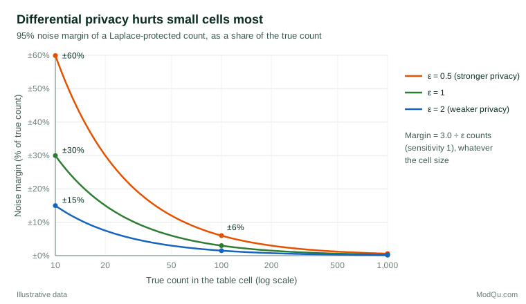
If the organisation then publishes the same counts split by age group, by tenure and by site, each additional table spends more budget. Five tables at ε = 1 each give a total of ε = 5. Keeping the total at 1 instead requires ε = 0.2 per table and a noise margin of about ±15 per cell. Planning which statistics matter most, before release, is therefore part of the method rather than an afterthought.
Differential privacy in practice: the 2020 census
The United States Census Bureau adopted differential privacy for the 2020 census, the largest application to date (Abowd, 2018). The decision exposed trade-offs that every data publisher faces. Abowd and Schmutte (2019) argue that privacy loss and statistical accuracy are both social goods and that the choice of ε is a policy decision, not a technical detail. Users of small-area data raised concerns: Kenny et al. (2021) found that the added noise could distort population counts for small and diverse areas used in electoral redistricting. Differential privacy makes the cost of protection explicit, which is uncomfortable but useful.
Practical guidance for survey and business data
- Treat confidentiality as a design requirement. Professional guidance places a duty on statisticians to protect the privacy of respondents and the confidentiality of their data (American Statistical Association, 2022). Decide what will be published, and in what detail, before fieldwork.
- Apply minimum cell sizes to all outputs, including dashboards, crosstabs and open-ended verbatims. Employee and customer surveys broken down by small teams, regions or rare segments are where disclosure most often happens in business settings.
- Watch for differencing. Two reports with slightly different filters can isolate one person by subtraction. Interactive tools that allow unlimited queries are the riskiest of all (Dinur & Nissim, 2003).
- Assess microdata against realistic linkage. Ask which quasi-identifiers an outsider could know, such as job title, postcode or exact dates, and coarsen them before sharing record-level data.
- Consider differential privacy for repeated or automated releases, where its composition property is most valuable, and report ε together with the expected noise so users can judge accuracy.
Limitations and common mistakes
- Equating de-identification with anonymity. Removing names leaves quasi-identifiers that can be linked (Sweeney, 2002; Rocher et al., 2019).
- Assuming aggregates are always safe. Enough accurate statistics can be reconstructed into records (Garfinkel et al., 2019).
- Treating ε as a quality score. A small ε is meaningless if the budget is spent many times over or if the sensitivity has been understated.
- Ignoring utility. Heavy suppression or noise can mislead, especially about small groups.
Key takeaways
Privacy protection in statistics is a trade-off between the risk that an individual is revealed and the accuracy of what is published. Traditional disclosure control, through thresholds, suppression, coarsening and synthetic data, remains the everyday toolkit. Differential privacy adds a provable guarantee, a single parameter that quantifies privacy loss, and a budget that tracks it across releases. Either way, plan outputs in advance, protect small cells and tell users how much noise protection adds.
References
Abowd, J. M. (2018). The U.S. Census Bureau adopts differential privacy. In Proceedings of the 24th ACM SIGKDD International Conference on Knowledge Discovery & Data Mining (p. 2867). ACM. https://doi.org/10.1145/3219819.3226070
Abowd, J. M., & Schmutte, I. M. (2019). An economic analysis of privacy protection and statistical accuracy as social choices. American Economic Review, 109(1), 171–202. https://doi.org/10.1257/aer.20170627
American Statistical Association. (2022). Ethical guidelines for statistical practice. American Statistical Association, Committee on Professional Ethics.
Dinur, I., & Nissim, K. (2003). Revealing information while preserving privacy. In Proceedings of the Twenty-Second ACM SIGMOD-SIGACT-SIGART Symposium on Principles of Database Systems (pp. 202–210). ACM. https://doi.org/10.1145/773153.773173
Drechsler, J. (2011). Synthetic datasets for statistical disclosure control: Theory and implementation. Springer. https://doi.org/10.1007/978-1-4614-0326-5
Dwork, C., McSherry, F., Nissim, K., & Smith, A. (2006). Calibrating noise to sensitivity in private data analysis. In S. Halevi & T. Rabin (Eds.), Theory of cryptography (pp. 265–284). Springer. https://doi.org/10.1007/11681878_14
Dwork, C., & Roth, A. (2014). The algorithmic foundations of differential privacy. Foundations and Trends in Theoretical Computer Science, 9(3–4), 211–487. https://doi.org/10.1561/0400000042
Erlingsson, Ú., Pihur, V., & Korolova, A. (2014). RAPPOR: Randomized aggregatable privacy-preserving ordinal response. In Proceedings of the 2014 ACM SIGSAC Conference on Computer and Communications Security (pp. 1054–1067). ACM. https://doi.org/10.1145/2660267.2660348
Garfinkel, S., Abowd, J. M., & Martindale, C. (2019). Understanding database reconstruction attacks on public data. Communications of the ACM, 62(3), 46–53. https://doi.org/10.1145/3287287
Hundepool, A., Domingo-Ferrer, J., Franconi, L., Giessing, S., Schulte Nordholt, E., Spicer, K., & de Wolf, P.-P. (2012). Statistical disclosure control. Wiley. https://doi.org/10.1002/9781118348239
Kenny, C. T., Kuriwaki, S., McCartan, C., Rosenman, E. T. R., Simko, T., & Imai, K. (2021). The use of differential privacy for census data and its impact on redistricting: The case of the 2020 U.S. Census. Science Advances, 7(41), Article eabk3283. https://doi.org/10.1126/sciadv.abk3283
Machanavajjhala, A., Kifer, D., Gehrke, J., & Venkitasubramaniam, M. (2007). l-diversity: Privacy beyond k-anonymity. ACM Transactions on Knowledge Discovery from Data, 1(1), Article 3. https://doi.org/10.1145/1217299.1217302
Narayanan, A., & Shmatikov, V. (2008). Robust de-anonymization of large sparse datasets. In 2008 IEEE Symposium on Security and Privacy (pp. 111–125). IEEE. https://doi.org/10.1109/SP.2008.33
Rocher, L., Hendrickx, J. M., & de Montjoye, Y.-A. (2019). Estimating the success of re-identifications in incomplete datasets using generative models. Nature Communications, 10(1), Article 3069. https://doi.org/10.1038/s41467-019-10933-3
Rubin, D. B. (1993). Discussion: Statistical disclosure limitation. Journal of Official Statistics, 9(2), 461–468.
Sweeney, L. (2002). k-anonymity: A model for protecting privacy. International Journal of Uncertainty, Fuzziness and Knowledge-Based Systems, 10(5), 557–570. https://doi.org/10.1142/S0218488502001648
Warner, S. L. (1965). Randomized response: A survey technique for eliminating evasive answer bias. Journal of the American Statistical Association, 60(309), 63–69. https://doi.org/10.1080/01621459.1965.10480775