
Statistics · Tests and models
Spatial Point Process Models for Event Location Knowledge
How spatial point process models analyse the locations of events such as crimes, store openings, disease cases or customer addresses, telling apart random scatter, clustering and regular spacing, and linking event intensity to local conditions.
Many data sets record not a value at a place, but the place itself. The addresses of customers who bought a product, the locations of road accidents, crimes, disease cases, new businesses, mobile phone complaints or trees in a forest are all collections of points on a map. The questions asked of such data are distinctive. Are the events clustered, or spread evenly? Is the rate of events higher near a factory, a motorway or a competitor's store? Does one event make others more likely nearby? Spatial point process models are the statistical tools built for these questions.
This article explains the basic ideas, the main summary statistics, the most common families of models and how they are fitted, with examples from market research, public health and crime analysis.
What makes point data different
In most spatial analysis, the locations are chosen by the researcher, such as weather stations or survey areas, and the interest lies in the values measured there. In a point pattern, the locations themselves are random and are the data. The number of points in any region is random too. A point process is a probability model for such patterns, describing how many points fall in any region and how they are arranged (Diggle, 2013; Illian et al., 2008).
Point pattern data are common in business even when they are not recognised as such. A retailer's loyalty card addresses form a point pattern of customers; a delivery company's failed deliveries form a pattern of problems; a city's store openings and closures over time form a spatio-temporal pattern. Treating such data as counts in arbitrary areas, such as postal districts, throws away information and can create artefacts depending on where the boundaries are drawn. Point process methods work directly with the locations.
Three basic patterns
Figure 1 shows the three reference patterns against which real data are usually compared.
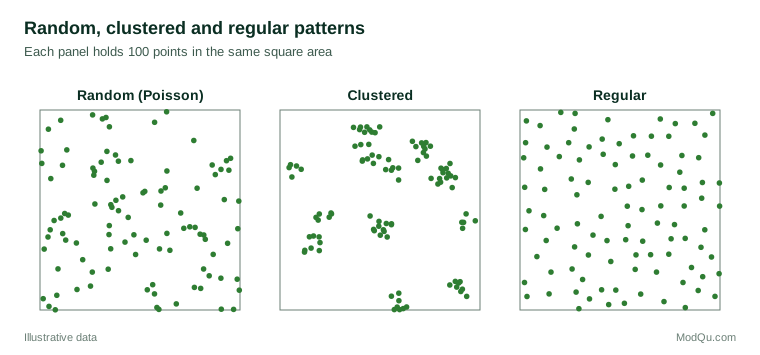
Complete spatial randomness is described by the homogeneous Poisson process. Points occur independently and with the same probability everywhere. This is the baseline model of "no structure". It is worth noting that random patterns do not look evenly spread to the human eye: they contain empty patches and small groups by chance, which is why visual judgement alone often finds clusters that are not there.
Clustered patterns have more points close together than randomness would produce. Clustering arises when events share a cause that varies over space, such as customers living near a store, or when events cause one another, such as aftershocks following an earthquake.
Regular patterns have fewer close pairs than randomness would produce, because points inhibit each other. Trees competing for light, shops of the same chain placed to avoid stealing each other's customers, and nesting birds defending territories all produce regular patterns.
Intensity: where events happen
The first property of a point process is its intensity, the expected number of events per unit area at each location. When intensity is the same everywhere, the process is homogeneous. In most real applications it is not: crimes are more frequent in city centres, and customers are more numerous where more people live.
Intensity can be estimated without a model by kernel smoothing, which places a small bump over each event and adds them up to give a smooth surface. The result depends on the width of the bump, called the bandwidth, which must be chosen with care. A common application is to compare two kernel estimates, for example the intensity of disease cases with the intensity of healthy controls drawn from the same population, giving a map of relative risk that is free of the population distribution (Kelsall & Diggle, 1995).
A modelling approach links intensity to explanatory variables. In an inhomogeneous Poisson process, the log intensity is a linear function of covariates such as population density, distance to a main road or average income. This model can be fitted with standard software for generalised linear models by placing a fine grid of dummy points over the study area, a technique due to Berman and Turner (1992). Diggle (1990) used this kind of model to test whether disease cases were concentrated near a specific point source of pollution, by letting intensity depend on distance from the source.
Second-order structure: are events clustered?
Intensity describes where events are expected. Second-order properties describe how events relate to each other. The most widely used summary is Ripley's K-function (Ripley, 1976, 1977). For a distance r, K(r) is the expected number of further events within distance r of a typical event, divided by the intensity. Under complete randomness, K(r) equals πr², the area of a circle of radius r. Values above this indicate clustering at that distance; values below indicate regularity.
Because K grows with the square of the distance, it is often transformed into the L-function, L(r) = √(K(r)/π), which equals r under randomness. Plotting L(r) − r gives a line that is flat at zero for a random pattern, rises above zero for clustering and falls below zero for regularity. Statistical significance is usually judged by simulating many random patterns with the same number of points and plotting the range of their L-functions as an envelope (Baddeley et al., 2015).
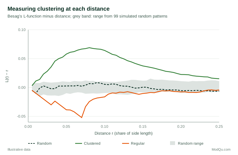
Figure 2 shows the result for the three patterns in Figure 1. The random pattern stays inside the grey band of simulated random patterns at all distances. The clustered pattern rises far above it, with the largest excess at a distance of about 0.08 of the side length, roughly the size of the clusters. The regular pattern falls below the band at distances up to about 0.07, the minimum spacing built into it. The L-function therefore says not only whether a pattern is clustered or regular, but at what scale.
An important caution is that the standard K-function assumes constant intensity. If intensity varies, for example because the population is concentrated in towns, events will appear clustered even if they occur independently. An inhomogeneous version of the K-function adjusts for estimated intensity, separating clustering caused by the population or other covariates from clustering caused by interaction between events (Baddeley et al., 2015).
Models for clustering
Two main families of model describe clustered patterns.
Cluster processes build clustering directly. In a Neyman–Scott process, first proposed to describe the distribution of galaxies (Neyman & Scott, 1958), unobserved "parent" points are scattered at random, and each parent produces a random number of "offspring" points scattered around it. The observed pattern consists of the offspring. The clustered pattern in Figure 1 was generated in this way. Such models are natural when events come in groups, such as customers belonging to the same household, or plants spreading from the same parent.
Cox processes produce clustering through a random intensity. The intensity surface is itself random, and given that surface, points follow a Poisson process. The most popular version is the log-Gaussian Cox process, in which the log intensity is a Gaussian random field (Møller et al., 1998). This model treats clustering as the result of unmeasured environmental factors that vary smoothly over space. It also links point processes to the wider field of geostatistics, in which Gaussian random fields are standard tools (Cressie, 1993; Diggle et al., 2013).
Fitting log-Gaussian Cox processes used to be slow, because the random field must be integrated over. Two developments made it routine. The integrated nested Laplace approximation (Rue et al., 2009) provides fast and accurate approximate Bayesian inference for latent Gaussian models, and the stochastic partial differential equation approach (Lindgren et al., 2011) represents a smooth random field efficiently on a triangular mesh. Simpson et al. (2016) showed how to combine these to fit log-Gaussian Cox processes directly to point locations, without first aggregating them onto a grid.
Models for regularity
Regular patterns call for Gibbs or Markov point processes, which specify how the presence of one point changes the probability of other points nearby. The Strauss process penalises each pair of points closer than a given distance (Strauss, 1975). With strong penalties, close pairs become rare and the pattern becomes regular; in the extreme, a "hard-core" process forbids pairs closer than the minimum distance altogether. Gibbs models are flexible and can include covariates, but their likelihood is difficult to compute, and they are usually fitted by pseudolikelihood or by simulation (Møller & Waagepetersen, 2003).
Self-exciting processes: events that trigger events
Some events make further events more likely in the near future and nearby. Earthquakes trigger aftershocks, burglaries are followed by repeat burglaries at the same or neighbouring addresses, and a viral social media post or a product complaint can trigger others. Self-exciting processes, introduced by Hawkes (1971) for events in time, model this directly: each event temporarily raises the intensity of further events.
Ogata (1988) developed the epidemic-type aftershock sequence model for earthquakes, in which each earthquake can trigger others in space and time. Mohler et al. (2011) applied the same idea to burglary data, showing that a self-exciting model predicted the locations of future crimes better than standard hot-spot maps, and the approach was later used in predictive policing software. For businesses, similar models can describe bursts of customer complaints, service outages or orders following a promotion, separating a background rate from the triggered excess.
Marks and time
Points often carry extra information, called marks. A customer location can be marked by spending, a crime by its type, a tree by its size and a store by whether it has closed. Marked point patterns raise new questions: are high-spending customers more clustered than low-spending ones, or do burglaries and car thefts occur in the same places? Mark correlation functions and cross-type versions of the K-function compare the arrangement of different kinds of points, for example measuring whether a chain's stores are closer to a competitor's stores than random placement would produce (Illian et al., 2008).
Many patterns also unfold over time, and adding time often makes the mechanism clearer. A cluster of complaints in one area within a single week may come from a single incident; the same cluster spread evenly over a year suggests a persistent local problem. Spatio-temporal point process models describe how intensity changes in both space and time and whether events are more likely to occur close together in both at once, which is the signature of contagion or triggering. Spatio-temporal log-Gaussian Cox processes have been used for real-time surveillance of disease, where a growing excess of cases in an area can trigger a public health response before an outbreak is obvious in raw counts (Diggle, 2013; Diggle et al., 2013). The same approach can monitor customer complaints, equipment faults or fraud reports, flagging areas where the current rate exceeds what the model expects given past patterns.
A worked example: customer locations
Consider a hypothetical chain with 20 stores in a metropolitan area that holds the home addresses of 15,000 loyalty card members. The marketing team wants to know where to target a leaflet campaign and whether there are areas of unexpectedly low membership.
A raw map of members shows concentrations around the stores and in densely populated suburbs. To separate these, an inhomogeneous Poisson model is fitted in which the log intensity of members depends on population density, distance to the nearest store, travel time by car and the share of households with children. The fitted model shows that intensity falls by about 30% for each additional 5 minutes of travel time, and is 40% higher in areas with more families.
The residuals of this model are then examined (Baddeley et al., 2005). The inhomogeneous L-function shows clustering at distances of up to about 300 metres beyond what the covariates explain, consistent with word-of-mouth between neighbours or with members of the same household signing up together. Fitting a log-Gaussian Cox process with these covariates gives a map of the remaining random intensity surface. Two areas stand out as having far fewer members than the covariates predict, despite being close to stores. On investigation, both are separated from the nearest store by a motorway with few crossings, a barrier that straight-line distance and the travel-time variable had not fully captured. These areas become priorities for targeted promotion, and the travel-time variable is refined.
Presence-only data and ecology
Point process models also resolve a long-standing problem in ecology. Species records often consist only of locations where a species was seen, with no record of where it was looked for and not found. Analysts used to invent "pseudo-absence" points to fit logistic regression. Warton and Shepherd (2010) showed that a Poisson point process model is the natural framework for such presence-only data, and that the popular pseudo-absence methods are approximations to it. Renner et al. (2015) give practical guidance. The same reasoning applies to market data that record only where customers are, without records of where non-customers live.
Software
The R package spatstat (Baddeley & Turner, 2005) provides tools for exploring, modelling and simulating point patterns, and is described in detail by Baddeley et al. (2015). Log-Gaussian Cox processes are commonly fitted with integrated nested Laplace approximations, and Bayesian models of many kinds can be fitted with general-purpose sampling software.
Practical guidance
- Define the study window carefully. Point process statistics depend on the area in which events could have occurred. Including lakes, parks or industrial zones where customers cannot live will make the pattern look more clustered than it is.
- Account for varying intensity first. Before concluding that events attract each other, model the effect of population and other covariates, then examine what clustering remains.
- Use edge corrections. Points near the boundary have neighbours outside the window that are not observed. Standard software corrects for this; ignoring it biases summary statistics.
- Judge significance by simulation. Compare the observed summary function with an envelope from simulated patterns under the null model, and remember that pointwise envelopes checked at many distances will exceed their limits by chance.
- Match the model to the mechanism. Cluster processes suit grouped events, Cox processes suit unmeasured environmental variation, Gibbs processes suit inhibition and self-exciting processes suit triggering.
- Check privacy. Exact home locations of customers or patients are personal data; analysis should use appropriate safeguards and published maps should not reveal individuals.
Limitations
Different mechanisms can produce the same pattern. A cluster process and a Cox process can have identical K-functions, and a single snapshot of points cannot tell whether events cluster because they share an environment or because they influence each other. Distinguishing the two often requires data over time, experimental variation or strong subject knowledge. Results also depend on the quality of the locations: geocoding errors, addresses recorded at postal-code centroids and missing records in some areas can all create apparent patterns. Finally, models assume that the observed points are complete within the study window. Under-reporting that varies by area, common in crime and disease data, will be mistaken for low intensity unless it is modelled.
Key takeaways
Spatial point process models treat event locations as data in their own right. Intensity describes where events are expected, and second-order summaries such as the K- and L-functions show whether events cluster or repel one another and at what distances. Poisson, cluster, Cox, Gibbs and self-exciting models each represent a different mechanism, and modern computational methods make them practical for large data sets. Used with careful study windows, adjustment for varying intensity and simulation-based checks, they turn maps of dots into knowledge about where events happen and why.
References
Baddeley, A., Rubak, E., & Turner, R. (2015). Spatial point patterns: Methodology and applications with R. Chapman and Hall/CRC. https://doi.org/10.1201/b19708
Baddeley, A., & Turner, R. (2005). spatstat: An R package for analyzing spatial point patterns. Journal of Statistical Software, 12(6), 1–42. https://doi.org/10.18637/jss.v012.i06
Baddeley, A., Turner, R., Møller, J., & Hazelton, M. (2005). Residual analysis for spatial point processes (with discussion). Journal of the Royal Statistical Society Series B: Statistical Methodology, 67(5), 617–666. https://doi.org/10.1111/j.1467-9868.2005.00519.x
Berman, M., & Turner, T. R. (1992). Approximating point process likelihoods with GLIM. Journal of the Royal Statistical Society Series C: Applied Statistics, 41(1), 31–38. https://doi.org/10.2307/2347614
Cressie, N. (1993). Statistics for spatial data (Rev. ed.). Wiley. https://doi.org/10.1002/9781119115151
Diggle, P. J. (1990). A point process modelling approach to raised incidence of a rare phenomenon in the vicinity of a prespecified point. Journal of the Royal Statistical Society Series A: Statistics in Society, 153(3), 349–362. https://doi.org/10.2307/2982977
Diggle, P. J. (2013). Statistical analysis of spatial and spatio-temporal point patterns (3rd ed.). Chapman and Hall/CRC. https://doi.org/10.1201/b15326
Diggle, P. J., Moraga, P., Rowlingson, B., & Taylor, B. M. (2013). Spatial and spatio-temporal log-Gaussian Cox processes: Extending the geostatistical paradigm. Statistical Science, 28(4), 542–563. https://doi.org/10.1214/13-STS441
Hawkes, A. G. (1971). Spectra of some self-exciting and mutually exciting point processes. Biometrika, 58(1), 83–90. https://doi.org/10.1093/biomet/58.1.83
Illian, J., Penttinen, A., Stoyan, H., & Stoyan, D. (2008). Statistical analysis and modelling of spatial point patterns. Wiley. https://doi.org/10.1002/9780470725160
Kelsall, J. E., & Diggle, P. J. (1995). Non-parametric estimation of spatial variation in relative risk. Statistics in Medicine, 14(21–22), 2335–2342. https://doi.org/10.1002/sim.4780142106
Lindgren, F., Rue, H., & Lindström, J. (2011). An explicit link between Gaussian fields and Gaussian Markov random fields: The stochastic partial differential equation approach. Journal of the Royal Statistical Society Series B: Statistical Methodology, 73(4), 423–498. https://doi.org/10.1111/j.1467-9868.2011.00777.x
Mohler, G. O., Short, M. B., Brantingham, P. J., Schoenberg, F. P., & Tita, G. E. (2011). Self-exciting point process modeling of crime. Journal of the American Statistical Association, 106(493), 100–108. https://doi.org/10.1198/jasa.2011.ap09546
Møller, J., Syversveen, A. R., & Waagepetersen, R. P. (1998). Log Gaussian Cox processes. Scandinavian Journal of Statistics, 25(3), 451–482. https://doi.org/10.1111/1467-9469.00115
Møller, J., & Waagepetersen, R. P. (2003). Statistical inference and simulation for spatial point processes. Chapman and Hall/CRC. https://doi.org/10.1201/9780203496930
Neyman, J., & Scott, E. L. (1958). Statistical approach to problems of cosmology. Journal of the Royal Statistical Society Series B: Statistical Methodology, 20(1), 1–29. https://doi.org/10.1111/j.2517-6161.1958.tb00272.x
Ogata, Y. (1988). Statistical models for earthquake occurrences and residual analysis for point processes. Journal of the American Statistical Association, 83(401), 9–27. https://doi.org/10.1080/01621459.1988.10478560
Renner, I. W., Elith, J., Baddeley, A., Fithian, W., Hastie, T., Phillips, S. J., Popovic, G., & Warton, D. I. (2015). Point process models for presence-only analysis. Methods in Ecology and Evolution, 6(4), 366–379. https://doi.org/10.1111/2041-210X.12352
Ripley, B. D. (1976). The second-order analysis of stationary point processes. Journal of Applied Probability, 13(2), 255–266. https://doi.org/10.2307/3212829
Ripley, B. D. (1977). Modelling spatial patterns. Journal of the Royal Statistical Society Series B: Statistical Methodology, 39(2), 172–192. https://doi.org/10.1111/j.2517-6161.1977.tb01615.x
Rue, H., Martino, S., & Chopin, N. (2009). Approximate Bayesian inference for latent Gaussian models by using integrated nested Laplace approximations. Journal of the Royal Statistical Society Series B: Statistical Methodology, 71(2), 319–392. https://doi.org/10.1111/j.1467-9868.2008.00700.x
Simpson, D., Illian, J. B., Lindgren, F., Sørbye, S. H., & Rue, H. (2016). Going off grid: Computationally efficient inference for log-Gaussian Cox processes. Biometrika, 103(1), 49–70. https://doi.org/10.1093/biomet/asv064
Strauss, D. J. (1975). A model for clustering. Biometrika, 62(2), 467–475. https://doi.org/10.1093/biomet/62.2.467
Warton, D. I., & Shepherd, L. C. (2010). Poisson point process models solve the "pseudo-absence problem" for presence-only data in ecology. The Annals of Applied Statistics, 4(3), 1383–1402. https://doi.org/10.1214/10-AOAS331