
Statistics · Tests and models
Multistate Models for Transition Process Knowledge
How multistate models describe movement between conditions over time, from trial to paying customer to churn or from health to illness, and how to estimate, check and use them.
Many processes are not a single journey from start to finish but a series of moves between conditions. A customer signs up for a trial, becomes a paying subscriber, goes quiet for a few months, returns, and eventually cancels. A patient moves from health to illness, possibly to recovery or relapse, and eventually to death. An employee moves between roles, takes leave and returns, and finally leaves the organisation. A survey panel member alternates between responding and not responding. Each of these is a transition process, and the questions people ask about them are about transitions: how quickly do people move from one state to another, what affects those moves, and where will a group of people be in a year's time?
Classical survival analysis answers a narrower question: how long until one event occurs? It treats life as two states, before and after the event. Multistate models generalise survival analysis to any number of states and any pattern of permitted transitions. They provide a single framework for competing risks, recurrent events, illness-death processes and customer life cycles, and they connect naturally to the Markov chain models long used in marketing. This article introduces the main ideas, the estimation methods, the key assumptions and the practical uses of multistate models in business and survey research.
States, transitions and the multistate diagram
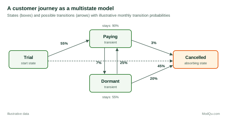
A multistate model starts with a diagram. Each box is a state, a condition a person can be in at a given time. Each arrow is a permitted transition. States from which no transitions lead out, such as death or account closure, are called absorbing; the others are transient. Figure 1 shows a simple customer journey with four states.
Several well-known models are special cases (Andersen & Keiding, 2002; Putter et al., 2007):
- The two-state survival model: alive to dead, or active to churned. Standard survival analysis applies.
- Competing risks: one initial state with several absorbing exits, such as a customer leaving because of price, service or relocation. Each exit is a different transition (Fine & Gray, 1999).
- The illness-death model: healthy, ill and dead, with transitions from healthy to ill, healthy to dead and ill to dead. It is the classic multistate model in medicine and has direct analogues in business, such as active, at-risk and churned.
- Recurrent and reversible models: states can be revisited, as with customers moving between active and dormant or panel members between responding and not responding.
The key quantities
Two kinds of quantity describe a multistate process.
Transition intensities (or hazards) describe the instantaneous rate of moving from state h to state j at time t, for someone currently in state h. They are the multistate version of the hazard function and are what regression models describe. A Cox model can be fitted separately for each transition, with its own covariate effects, so that, for example, the effect of price on moving from paying to dormant can differ from its effect on moving from dormant to cancelled (Cox, 1972; Therneau & Grambsch, 2000).
Transition probabilities describe the probability of being in state j at a later time t, given being in state h at an earlier time s. They combine the effects of all the paths between the two states, including detours. From them come the state occupation probabilities: the share of a cohort expected to be in each state at each time. These are usually the quantities that decision-makers want: how many of this month's trial customers will still be paying in a year?
In a Markov model, the transition probabilities can be calculated from the intensities by a product integral, and their nonparametric estimate, the Aalen-Johansen estimator, generalises the Kaplan-Meier estimator to several states (Kaplan & Meier, 1958; Aalen et al., 2008).
A simple illness-death illustration
The value of separating transitions is easiest to see in the illness-death model. Suppose a hypothetical study follows 10,000 employees and records when they first take long-term sick leave and when they leave the organisation. A standard survival analysis of leaving would treat everyone the same until they leave, perhaps with a time-varying indicator for sick leave. A multistate model instead estimates three transitions: well to sick leave, well to leaving and sick leave to leaving. The analysis might show that the rate of leaving is three times higher during and after sick leave, and that factors such as workload mainly affect the move into sick leave, while factors such as manager support mainly affect whether people on sick leave return or leave. Those are different levers, and an organisation would miss the distinction if it modelled only time to leaving.
Regression on transitions
Covariates enter a multistate model through the transition intensities. The simplest approach fits a separate proportional hazards model to each transition, which allows every covariate to have a different effect on every move. With many transitions and few events, that can use up the data quickly, so analysts often constrain effects to be equal across similar transitions, for example the effect of age on any move into an absorbing state, or assume proportional baseline intensities for related transitions (Putter et al., 2007). These choices should be guided by subject-matter reasoning and tested, just as with any regression model.
The Markov assumption
Most multistate models assume that the process is Markov: the future depends only on the current state and the current time, not on how the person got there or how long they have been in the current state. Under this assumption, a customer who has been paying for two years and one who has just become paying have the same chances of moving next month, provided that time is measured in the same way for both.
The assumption is convenient, but it is often questionable. Customers who have been dormant for one month probably reactivate more readily than those dormant for a year. Several relaxations are available:
- Semi-Markov (clock-reset) models measure time since entry into the current state, so that intensities can depend on how long someone has been there (Meira-Machado et al., 2009).
- History covariates, such as the number of previous dormant spells, can be added to transition models.
- Landmark methods estimate transition probabilities without assuming the Markov property, by analysing only the people in a given state at a chosen time (Putter & Spitoni, 2018). Datta and Satten (2001) showed that the Aalen-Johansen estimator of state occupation probabilities remains valid even for non-Markov processes when censoring is independent, though transition probabilities from intermediate states may not be.
Checking the Markov assumption, for instance by adding time-in-state to each transition model and testing whether it matters, is a basic diagnostic (Titman & Sharples, 2010).
Continuous time and panel data
How a process is observed shapes how it can be modelled.
Continuously observed data record the exact time of each transition. Subscription systems and electronic records often provide this. Each transition can then be modelled with standard survival methods, treating the time at risk for transition h → j as starting when someone enters state h and being censored when they move to another state or leave observation. This approach is set out by Andersen et al. (1993) using counting process theory, with the time-varying extension of the Cox model by Andersen and Gill (1982) as a building block, and is implemented in software such as the R package mstate (de Wreede et al., 2011).
Panel data record only the state at a series of visits: a survey wave every six months, a quarterly account review, a clinic appointment. The exact transition times, and sometimes whole visits to intermediate states, are unknown. Kalbfleisch and Lawless (1985) showed how to estimate continuous-time Markov models from such data by maximum likelihood, using the matrix exponential to link intensities to the probabilities of moving between observed states over each interval. The R package msm implements this approach and is widely used for panel data (Jackson, 2011). For longitudinal surveys, this is often the only appropriate approach, since respondents' states are known only at each wave.
Multistate models and Markov chains in marketing
Marketing researchers have long modelled customer relationships as Markov chains, in which customers move each period between states defined by recency, frequency or activity. Pfeifer and Carraway (2000) showed how such chains can be used to calculate customer lifetime value by combining transition probabilities with the profit earned in each state, and Gupta et al. (2006) review the wider family of lifetime value models. Discrete-time Markov chains are multistate models observed at regular intervals, so the two traditions share a common foundation.
When states are not directly observed, for example a customer's underlying level of engagement, hidden Markov models infer them from observed behaviour (Netzer et al., 2008; Zucchini et al., 2016). Latent transition analysis plays the same role for categorical survey responses, describing how respondents move between latent classes such as attitude types between waves (Collins & Lanza, 2009). These latent-state models extend the multistate idea to situations where the state itself must be measured.
A worked example: projecting a subscription cohort
Return to the customer journey in Figure 1 and suppose that monthly transition probabilities have been estimated from the account histories of a hypothetical streaming service. Each month, 90% of paying customers continue to pay, 7% go dormant and 3% cancel; 25% of dormant customers return to paying, 55% stay dormant and 20% cancel; and at the end of the one-month trial, 55% convert to paying and 45% cancel.
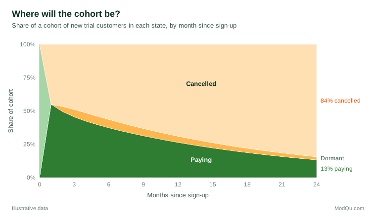
Multiplying the matrix of transition probabilities month by month gives the state occupation probabilities for a cohort of trial customers (Figure 2). After one month, 55% are paying. By month 12, about 26% are paying, 5% are dormant and 69% have cancelled. By month 24, about 13% are paying and 84% have cancelled.
This projection supports several decisions that a single churn rate cannot:
- Revenue forecasting. Multiplying the expected number of paying customers in each month by the monthly price gives expected revenue per cohort, the basis of lifetime value (Fader & Hardie, 2007).
- Targeting the right transition. The model shows that a two-percentage-point improvement in the dormant-to-paying probability, from 25% to 27%, raises the 24-month paying share less than a one-point cut in the paying-to-dormant probability, because many more customers pass through the paying state. Interventions can be prioritised accordingly.
- Covariate effects by transition. Fitting separate models for each transition might show that a price increase raises paying-to-dormant moves but has little effect on dormant-to-cancelled moves, while service problems do the reverse. A single churn model would blend these into one coefficient.
Real applications would replace fixed monthly probabilities with intensities that depend on covariates and on time since sign-up, and would report uncertainty, for example by bootstrapping customers and recomputing the projection.
Applications beyond customers
The same tools apply across ModQu's areas of work.
- Survey panels. States can be responding, temporarily non-responding and permanently lost. A multistate model shows not only how many members leave but how many return after missing a wave, which informs fieldwork strategies and weighting.
- Employment and careers. Employer surveys and administrative records can be modelled as moves between employment, unemployment, training and inactivity, revealing whether training shortens unemployment spells or simply delays exits.
- Health and wellbeing. Epidemiology has been the main home of multistate models, used for disease progression, disability and recovery (Commenges, 1999; Hougaard, 1999).
- Credit and collections. Accounts move between current, early arrears, late arrears, recovery and write-off; transition models underpin provisioning and collection strategies.
Comparing multistate models with other approaches
| Question | Typical simple approach | What a multistate model adds |
|---|---|---|
| How long until customers churn? | Kaplan-Meier curve or Cox model for time to cancellation | Separate rates for moving into and out of intermediate states such as dormancy |
| Why do customers leave? | Logistic regression on a churn flag | Covariate effects specific to each transition and each exit route |
| How many will be active next year? | Apply an average retention rate | Projected occupation of every state, accounting for returns and detours |
| Do panel members return after missing a wave? | Count re-entrants | Rates of return as a function of time away and member characteristics |
The table is a reminder that multistate models are not a replacement for simpler tools but an extension of them. If customers never return from dormancy and there is only one way to leave, a standard survival model is the multistate model. The extra structure pays off when processes are reversible, when there are several exits or when intermediate states carry information about what happens next.
Estimation in practice
A typical analysis proceeds in five steps.
- Define the states and transitions with the business or scientific question in mind. Too many states fragment the data; too few hide important distinctions. Each state should be clearly measurable from the available data.
- Prepare the data in long format, with one row per person per transition at risk, recording entry time, exit time and whether the transition occurred. This is the form expected by most software (de Wreede et al., 2011).
- Estimate transition intensities, first nonparametrically to see the patterns, then with regression models for covariates. Decide whether effects should be shared across transitions or estimated separately.
- Check assumptions: the Markov property, proportional hazards within each transition and the independence of censoring (Titman & Sharples, 2010).
- Compute and communicate state occupation probabilities, ideally for a few representative customer or patient profiles, with uncertainty bands.
Communicating results
Multistate results can overwhelm an audience with transition matrices and hazard ratios. Three formats usually work better. First, the state diagram itself, annotated with the size of each flow over a meaningful period, such as the number of customers who moved along each arrow last quarter. Second, stacked state occupation charts like Figure 2 for a few representative profiles, for example a typical customer on a monthly plan and a typical customer on an annual plan. Third, scenario comparisons that show how state occupation at a chosen horizon changes if one transition probability is improved, which links the model directly to the decision at hand.
Each of these should carry an indication of uncertainty. Intervals for state occupation probabilities can be obtained by simulation from the estimated model or by bootstrapping individuals and refitting. A projection that shows 26% of a cohort still paying at month 12, with an interval from 23% to 29%, gives a planner something to work with; a single number invites false precision.
Limitations and common mistakes
- Treating competing events as censoring. If customers who switch to a competitor are simply censored in an analysis of cancellations for price reasons, the cumulative probability of price cancellations will be overestimated. Competing exits must be modelled as separate transitions (Putter et al., 2007).
- Ignoring re-entry. Treating the first dormant spell as the end of the customer relationship overstates loss when many dormant customers return.
- Assuming Markov without checking. Duration in state often matters. Where it does, semi-Markov or landmark approaches give more realistic projections.
- Sparse transitions. Rare transitions, such as from cancelled back to paying in a model that allows win-backs, may have too few events to estimate covariate effects reliably. Combining or constraining them can help.
- Misreading panel data. When states are observed only at waves, moves between waves can be missed. Treating the observed states as if transitions happened exactly at the wave dates biases intensities; continuous-time panel methods avoid this (Kalbfleisch & Lawless, 1985).
- Over-interpreting intensities. A covariate's effect on one transition intensity does not translate simply into its effect on the probability of being in a state later. Report effects on state occupation probabilities as well (Andersen & Keiding, 2002).
Key takeaways
Multistate models treat a process as movement between states, with each permitted transition having its own rate and its own drivers. They unify survival analysis, competing risks, illness-death models and Markov chain models of customer relationships, and they can be estimated from continuously observed histories or from panel data collected at waves. Their outputs, from transition-specific effects to projected state occupation for a cohort, answer the questions organisations actually ask: where will our customers, patients or panel members be, and which transition should we try to change? Used with careful definition of states, checks of the Markov assumption and honest reporting of uncertainty, they turn event histories into rich knowledge about how processes unfold.
References
Aalen, O. O., Borgan, Ø., & Gjessing, H. K. (2008). Survival and event history analysis: A process point of view. Springer. https://doi.org/10.1007/978-0-387-68560-1
Andersen, P. K., Borgan, Ø., Gill, R. D., & Keiding, N. (1993). Statistical models based on counting processes. Springer. https://doi.org/10.1007/978-1-4612-4348-9
Andersen, P. K., & Gill, R. D. (1982). Cox's regression model for counting processes: A large sample study. The Annals of Statistics, 10(4), 1100–1120. https://doi.org/10.1214/aos/1176345976
Andersen, P. K., & Keiding, N. (2002). Multi-state models for event history analysis. Statistical Methods in Medical Research, 11(2), 91–115. https://doi.org/10.1191/0962280202SM276ra
Collins, L. M., & Lanza, S. T. (2009). Latent class and latent transition analysis: With applications in the social, behavioral, and health sciences. Wiley. https://doi.org/10.1002/9780470567333
Commenges, D. (1999). Multi-state models in epidemiology. Lifetime Data Analysis, 5(4), 315–327. https://doi.org/10.1023/A:1009636125294
Cox, D. R. (1972). Regression models and life-tables. Journal of the Royal Statistical Society Series B: Statistical Methodology, 34(2), 187–202. https://doi.org/10.1111/j.2517-6161.1972.tb00899.x
Datta, S., & Satten, G. A. (2001). Validity of the Aalen–Johansen estimators of stage occupation probabilities and Nelson–Aalen estimators of integrated transition hazards for non-Markov models. Statistics & Probability Letters, 55(4), 403–411. https://doi.org/10.1016/S0167-7152(01)00155-9
de Wreede, L. C., Fiocco, M., & Putter, H. (2011). mstate: An R package for the analysis of competing risks and multi-state models. Journal of Statistical Software, 38(7), 1–30. https://doi.org/10.18637/jss.v038.i07
Fader, P. S., & Hardie, B. G. S. (2007). How to project customer retention. Journal of Interactive Marketing, 21(1), 76–90. https://doi.org/10.1002/dir.20074
Fine, J. P., & Gray, R. J. (1999). A proportional hazards model for the subdistribution of a competing risk. Journal of the American Statistical Association, 94(446), 496–509. https://doi.org/10.1080/01621459.1999.10474144
Gupta, S., Hanssens, D., Hardie, B., Kahn, W., Kumar, V., Lin, N., Ravishanker, N., & Sriram, S. (2006). Modeling customer lifetime value. Journal of Service Research, 9(2), 139–155. https://doi.org/10.1177/1094670506293810
Hougaard, P. (1999). Multi-state models: A review. Lifetime Data Analysis, 5(3), 239–264. https://doi.org/10.1023/A:1009672031531
Jackson, C. H. (2011). Multi-state models for panel data: The msm package for R. Journal of Statistical Software, 38(8), 1–28. https://doi.org/10.18637/jss.v038.i08
Kalbfleisch, J. D., & Lawless, J. F. (1985). The analysis of panel data under a Markov assumption. Journal of the American Statistical Association, 80(392), 863–871. https://doi.org/10.1080/01621459.1985.10478195
Kaplan, E. L., & Meier, P. (1958). Nonparametric estimation from incomplete observations. Journal of the American Statistical Association, 53(282), 457–481. https://doi.org/10.1080/01621459.1958.10501452
Meira-Machado, L., de Uña-Álvarez, J., Cadarso-Suárez, C., & Andersen, P. K. (2009). Multi-state models for the analysis of time-to-event data. Statistical Methods in Medical Research, 18(2), 195–222. https://doi.org/10.1177/0962280208092301
Netzer, O., Lattin, J. M., & Srinivasan, V. (2008). A hidden Markov model of customer relationship dynamics. Marketing Science, 27(2), 185–204. https://doi.org/10.1287/mksc.1070.0294
Pfeifer, P. E., & Carraway, R. L. (2000). Modeling customer relationships as Markov chains. Journal of Interactive Marketing, 14(2), 43–55. https://doi.org/10.1002/(SICI)1520-6653(200021)14:2<43::AID-DIR4>3.0.CO;2-H
Putter, H., Fiocco, M., & Geskus, R. B. (2007). Tutorial in biostatistics: Competing risks and multi-state models. Statistics in Medicine, 26(11), 2389–2430. https://doi.org/10.1002/sim.2712
Putter, H., & Spitoni, C. (2018). Non-parametric estimation of transition probabilities in non-Markov multi-state models: The landmark Aalen–Johansen estimator. Statistical Methods in Medical Research, 27(7), 2081–2092. https://doi.org/10.1177/0962280216674497
Therneau, T. M., & Grambsch, P. M. (2000). Modeling survival data: Extending the Cox model. Springer. https://doi.org/10.1007/978-1-4757-3294-8
Titman, A. C., & Sharples, L. D. (2010). Model diagnostics for multi-state models. Statistical Methods in Medical Research, 19(6), 621–651. https://doi.org/10.1177/0962280209105541
Zucchini, W., MacDonald, I. L., & Langrock, R. (2016). Hidden Markov models for time series: An introduction using R (2nd ed.). Chapman and Hall/CRC. https://doi.org/10.1201/b20790