
Statistics · Tests and models
Spatial Autoregressive Models for Dependent Geographic Knowledge
How spatial autoregressive models handle data from neighbouring regions that are not independent, how to read their spillover effects, and when simpler approaches are enough.
Data collected across places rarely behave like independent observations. House prices in one neighbourhood track prices next door, unemployment spreads across commuting zones, and a retailer's sales in one postal area depend partly on what happens in surrounding areas. Tobler (1970) summarised the pattern in what is often called the first law of geography: everything is related to everything else, but near things are more related than distant things. Ordinary regression assumes the opposite, that each observation is independent. When that assumption fails, standard errors are wrong, coefficients can be biased and important spillover effects go unmeasured. Spatial autoregressive models were developed to deal with this.
Measuring spatial dependence
The first step is to define who is a neighbour. A spatial weights matrix W records, for each pair of areas, whether and how strongly they are connected: sharing a border, lying within a set distance, or being among the k nearest. Rows are usually standardised to sum to one, so that Wy is the average value among each area's neighbours, called the spatial lag.
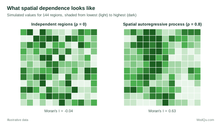
Moran's I, proposed by Moran (1950), measures overall spatial autocorrelation by comparing each area's deviation from the mean with that of its neighbours. Values near zero indicate no pattern; positive values indicate clustering of similar values. Local versions identify where clusters and outliers occur (Anselin, 1995). Figure 1 shows the difference between independent values and values generated by a spatial process.
The main model family
Spatial econometrics, developed by Anselin (1988) and others from earlier work on lattice models (Besag, 1974; Ord, 1975), offers several related models.
The spatial lag (SAR) model lets the outcome in each area depend directly on outcomes in neighbouring areas:
y = ρWy + Xβ + ε
The parameter ρ measures the strength of spatial dependence. This model suits processes with genuine interaction, such as competing prices or the spread of adoption.
The spatial error model (SEM) places dependence in the error term instead: y = Xβ + u, with u = λWu + ε. It suits situations where unmeasured factors, such as local climate or culture, are themselves spatially clustered, but outcomes do not directly influence each other.
The spatial Durbin model adds the neighbours' explanatory variables, WX, to the lag model. LeSage and Pace (2009) argue that it is a sensible default because it nests several simpler models and remains unbiased under a wider range of true processes. A model with only WX terms (often called SLX) is a simpler alternative that avoids feedback loops (Elhorst, 2014).
Because the spatial lag Wy is correlated with the error term, ordinary least squares is biased for the lag model. Estimation uses maximum likelihood (Ord, 1975), generalised method of moments or instrumental variables (Kelejian & Prucha, 1998), or Bayesian methods (LeSage & Pace, 2009).
Interpreting spillovers
A coefficient in a spatial lag model is not the effect of the variable. Because each area affects its neighbours, which affect their neighbours in turn, a change ripples outwards and returns. Solving the model gives y = (I − ρW)−1(Xβ + ε), and the matrix (I − ρW)−1 spreads every change across the map. With row-standardised weights, the average total effect of a variable is roughly β/(1 − ρ). With ρ = 0.8, that is five times the coefficient.
LeSage and Pace (2009) therefore recommend reporting three summary measures for each variable:
- the direct effect, the average effect of a change in an area on its own outcome, including feedback through neighbours;
- the indirect effect, or spillover, the average effect on all other areas;
- the total effect, their sum.
A worked example: store sales and local income
Consider a hypothetical retailer with stores in 400 postal areas. A regression of sales per household on local median income, population density and competitor count shows clear spatial clustering in the residuals (Moran's I about 0.35), so a spatial Durbin model is fitted with weights based on the five nearest areas.
Suppose the estimated ρ is 0.45 and the direct effect of a 10% rise in local income is a 3.0% rise in sales, while the indirect effect is a further 2.0%, because higher incomes in neighbouring areas also draw shoppers into the store's area. The total effect, 5.0%, is much larger than the ordinary regression coefficient would suggest, and the spillover changes how the retailer should read regional growth: income growth in surrounding districts matters almost as much as growth in the store's own area. In this illustration, the competitor count has a negative direct effect but a small positive indirect effect, consistent with competitors pulling some shoppers away while also drawing traffic to a shopping area.
Choosing between lag and error models
Analysts often start from an ordinary regression and use diagnostic tests to decide which spatial model is needed. Lagrange multiplier tests, computed from the ordinary least squares residuals, test separately for an omitted spatial lag and for spatially correlated errors, and robust versions of each test allow for the presence of the other (Anselin, 1988). If only the error test is significant, a spatial error model is indicated; if only the lag test is, a lag model. When both are significant, the spatial Durbin model is a reasonable compromise, because it nests both and can be simplified if the data support a restriction (LeSage & Pace, 2009; Elhorst, 2014).
The choice is not only statistical. The two models answer different questions. An error model treats spatial dependence as a nuisance that must be accounted for to get correct standard errors, and its coefficients keep their usual meaning. A lag model treats dependence as part of the process being studied, with spillovers that are of interest in themselves. Survey researchers comparing regional estimates often need only the first; analysts studying how prices, adoption or opinions spread between places need the second.
Spatial models in survey and market research
Survey estimates for small areas are themselves spatially correlated, because neighbouring areas share demographics, media markets and economic conditions. Spatial models can borrow strength from neighbours to improve estimates for areas with few respondents, an approach that links spatial statistics to small area estimation. In market research, spatial lag models describe how the presence of a store, a competitor or a promotion in one area affects demand in surrounding areas, which matters for site selection and for evaluating local campaigns.
Practical guidance
- Test residuals first. Map the residuals of an ordinary model and compute Moran's I. If there is no spatial dependence, a simpler model is enough.
- Choose weights with care and test alternatives. Contiguity, distance bands and nearest-neighbour weights embody different assumptions about how places interact. Results that change sharply with the weights matrix should be reported with caution.
- Report effects, not coefficients. In lag and Durbin models, present direct, indirect and total effects with their uncertainty.
- Match the model to the theory. Ask whether outcomes truly influence each other (lag), whether unmeasured factors cluster (error), or whether neighbours' characteristics matter (SLX).
- Use good tools. Open-source software makes weights construction, testing and estimation routine (Bivand et al., 2013).
Limitations and common mistakes
Spatial models are easy to fit and easy to over-interpret. Gibbons and Overman (2012) criticise the common practice of treating the spatial lag coefficient as evidence of causal spillovers: many different processes produce the same spatial correlation, and the models identify causal effects only under strong assumptions. This is a spatial version of the reflection problem described by Manski (1993), in which group averages and individual outcomes cannot easily be separated. Other common mistakes include ignoring the scale at which areas are defined, since boundaries chosen for administrative convenience can create or hide patterns, and reading spatial dependence that is in fact caused by a missing variable as interaction between places. For prediction rather than explanation, geostatistical methods (Cressie, 1993) and geographically weighted regression (Brunsdon et al., 1996) are useful alternatives.
Key takeaways
Geographic data are dependent by nature, and ignoring that dependence misstates uncertainty and misses spillovers. Spatial autoregressive models use a weights matrix to describe how places are connected and estimate how strongly outcomes or errors spread between neighbours. Their coefficients must be translated into direct, indirect and total effects before they mean anything to a decision-maker. Used with tested weights, appropriate model choice and caution about causal claims, they turn maps of correlated numbers into knowledge about how places influence one another.
References
Anselin, L. (1988). Spatial econometrics: Methods and models. Kluwer Academic. https://doi.org/10.1007/978-94-015-7799-1
Anselin, L. (1995). Local indicators of spatial association—LISA. Geographical Analysis, 27(2), 93–115. https://doi.org/10.1111/j.1538-4632.1995.tb00338.x
Besag, J. (1974). Spatial interaction and the statistical analysis of lattice systems. Journal of the Royal Statistical Society Series B: Statistical Methodology, 36(2), 192–225. https://doi.org/10.1111/j.2517-6161.1974.tb00999.x
Bivand, R. S., Pebesma, E., & Gómez-Rubio, V. (2013). Applied spatial data analysis with R (2nd ed.). Springer. https://doi.org/10.1007/978-1-4614-7618-4
Brunsdon, C., Fotheringham, A. S., & Charlton, M. E. (1996). Geographically weighted regression: A method for exploring spatial nonstationarity. Geographical Analysis, 28(4), 281–298. https://doi.org/10.1111/j.1538-4632.1996.tb00936.x
Cressie, N. (1993). Statistics for spatial data (Rev. ed.). Wiley. https://doi.org/10.1002/9781119115151
Elhorst, J. P. (2014). Spatial econometrics: From cross-sectional data to spatial panels. Springer. https://doi.org/10.1007/978-3-642-40340-8
Gibbons, S., & Overman, H. G. (2012). Mostly pointless spatial econometrics? Journal of Regional Science, 52(2), 172–191. https://doi.org/10.1111/j.1467-9787.2012.00760.x
Kelejian, H. H., & Prucha, I. R. (1998). A generalized spatial two-stage least squares procedure for estimating a spatial autoregressive model with autoregressive disturbances. The Journal of Real Estate Finance and Economics, 17(1), 99–121. https://doi.org/10.1023/A:1007707430416
LeSage, J., & Pace, R. K. (2009). Introduction to spatial econometrics. Chapman and Hall/CRC. https://doi.org/10.1201/9781420064254
Manski, C. F. (1993). Identification of endogenous social effects: The reflection problem. The Review of Economic Studies, 60(3), 531–542. https://doi.org/10.2307/2298123
Moran, P. A. P. (1950). Notes on continuous stochastic phenomena. Biometrika, 37(1–2), 17–23. https://doi.org/10.1093/biomet/37.1-2.17
Ord, K. (1975). Estimation methods for models of spatial interaction. Journal of the American Statistical Association, 70(349), 120–126. https://doi.org/10.1080/01621459.1975.10480272
Tobler, W. R. (1970). A computer movie simulating urban growth in the Detroit region. Economic Geography, 46(Suppl. 1), 234–240. https://doi.org/10.2307/143141