
Statistics · Tests and models
Joint Modeling of Longitudinal and Survival Outcomes for Integrated Knowledge
How joint models link repeated measurements, such as engagement scores or biomarkers, to the timing of events such as churn or illness, and why analysing the two separately can mislead.
Many important questions involve two kinds of data collected on the same people over time. A subscription business records each customer's monthly engagement and also whether and when the customer cancels. A clinical study measures a biomarker at every visit and also records when patients experience an event such as relapse. A panel survey tracks respondents' attitudes wave after wave and also notes when they drop out. In each case there is a longitudinal outcome, measured repeatedly, and a time-to-event outcome, observed once and often censored.
The two are usually connected. Falling engagement is a warning sign of churn; a rising biomarker signals disease progression; disengaged panel members are more likely to leave. Analysing each outcome on its own throws away that connection and can produce biased answers. Joint models analyse both together, using a shared structure that links the trajectory of the repeated measurements to the risk of the event. This article explains why joint modelling is needed, how the models are built and what they offer for prediction and decision-making.
Why separate analyses fall short
Using the repeated measurement to explain the event
The natural first approach is a Cox proportional hazards model (Cox, 1972) with the repeated measurement entered as a time-varying covariate, a standard extension of the model (Andersen & Gill, 1982; Therneau & Grambsch, 2000). This works well for covariates that are measured without error and are known at every moment, such as calendar time or contract type. Engagement scores and biomarkers are different in three ways.
- They are measured with error. A single month's score is a noisy reading of a customer's underlying engagement. Using noisy values as covariates biases the estimated association towards zero, a problem identified for failure-time models by Prentice (1982).
- They are measured only at certain times. The Cox model needs the covariate value at every event time, so analysts carry the last observation forward, which ignores change since the last measurement.
- They are endogenous: the measurement process stops when the event happens. A customer who cancels has no engagement score afterwards. Such covariates do not satisfy the conditions under which the time-varying Cox model has its usual interpretation (Rizopoulos, 2012).
Using the event to explain the repeated measurement
The reverse problem arises when the main interest is in the trajectory. Mixed-effects models (Laird & Ware, 1982) and generalised estimating equations (Liang & Zeger, 1986) are the standard tools for repeated measurements. Both assume that missing measurements are ignorable. When people leave a study because of the very process being measured, the remaining measurements over-represent those who are doing well, and the dropout is informative (Diggle & Kenward, 1994). In Rubin's (1976) terms, the missing data are not missing at random, and an analysis that ignores the dropout process gives biased trajectories (Little & Rubin, 2019).
How a joint model is built
A joint model has two submodels connected by a shared component (Figure 1).
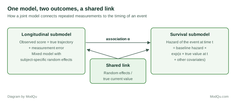
The longitudinal submodel is usually a linear mixed model. Each person's observed value at time t equals their true value mi(t) plus measurement error, and the true value follows a trajectory with person-specific random intercepts and slopes:
yi(t) = mi(t) + εi(t), mi(t) = (β0 + b0i) + (β1 + b1i)t
The survival submodel is a proportional hazards model in which the hazard at time t depends on the true, error-free value at that moment:
hi(t) = h0(t) exp(γ′wi + α mi(t))
Here wi are baseline covariates and α measures how strongly the current underlying level is associated with the risk of the event. Because both submodels share the random effects bi, the parameters are estimated together, by maximum likelihood or Bayesian methods, and each part of the data informs the other.
This "current value" formulation was introduced by Faucett and Thomas (1996) and Wulfsohn and Tsiatis (1997). Henderson et al. (2000) proposed a more general framework in which the two submodels are linked through correlated latent processes. Other association structures are possible: the hazard may depend on the slope of the trajectory (how fast engagement is falling), on the area under it (cumulative exposure) or directly on the random effects. Joint latent class models replace the continuous link with a small number of latent groups, each with its own trajectory and risk profile (Proust-Lima et al., 2014).
What joint models deliver
Unbiased association estimates
By modelling the true trajectory rather than noisy observed values, joint models correct the attenuation caused by measurement error and use all available measurements, not only the most recent. Simulation studies and applications in medicine show that the estimated association between the marker and the event is typically stronger, and more accurate, than in a time-varying Cox model with observed values (Ibrahim et al., 2010).
Trajectories that account for dropout
Because the event process is modelled jointly, the estimated average trajectory in the longitudinal submodel is adjusted for informative dropout, under the assumption that dropout depends on the true trajectory. This is a form of selection model for missing data, and it is often more realistic than assuming that people leave at random.
Dynamic, individual predictions
The most practical output is dynamic prediction. For a person still at risk at time t, the model combines all of their measurements so far to estimate their current trajectory and then computes the probability that they will remain event-free for a further period. Each new measurement updates the prediction (Rizopoulos, 2011).
Figure 2 illustrates the idea with two hypothetical subscribers. Both start with similar engagement. Customer A stays level; customer B declines steadily over six months. At month 6, the joint model projects each customer's trajectory and converts it into a retention curve. Customer A has about a 92% chance of still being subscribed at month 12 and 85% at month 18. Customer B, whose engagement is projected to keep falling, has about 65% at month 12 and only 17% at month 18.
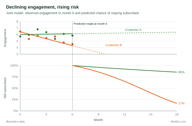
A retention team could use such predictions to prioritise outreach, and the predictions would sharpen every month as new engagement data arrived. Rizopoulos (2011) also describes how to measure the accuracy of such predictions over time, using time-dependent discrimination and calibration measures, so that the model's usefulness can be checked before it guides action.
A worked example: panel attrition and attitude change
Consider a hypothetical online panel that measures trust in institutions every quarter for three years. Some members stop responding. A mixed model fitted only to the responses shows trust falling by 0.10 points per year on a 10-point scale. The analyst suspects that members whose trust is falling fastest are also the most likely to disengage from a panel about public life.
A joint model with a current-value association finds that each one-point lower level of underlying trust is associated with a 25% higher hazard of leaving the panel (hazard ratio about 1.25 per point lower). Accounting for this informative attrition, the estimated average decline in trust is steeper, about 0.16 points per year, because the members who left were on worse trajectories than those who stayed. The separate analysis understated the decline by more than a third. In this illustration the joint model changes a substantive conclusion, and it also produces a model of attrition risk that the panel managers can use to target retention incentives.
Where joint models fit in business and survey research
Joint models are most associated with medicine, where they were developed to link markers such as CD4 counts or tumour size to survival. The same structure appears wherever an organisation follows units over time and cares about an event.
- Customer analytics. Usage, satisfaction scores, complaint counts or payment behaviour, measured monthly, can be linked to cancellation, default or upgrade.
- Employee research. Repeated engagement survey scores can be linked to the timing of resignations, giving a sharper estimate of how engagement relates to retention than a single annual snapshot.
- Longitudinal surveys and panels. Repeated answers can be linked to attrition, correcting trajectories for informative dropout and helping managers identify members at risk of leaving.
- Product reliability. Repeated sensor readings or performance measures can be linked to the time of failure, supporting maintenance planning.
In each setting the key questions are the same: is the event related to the level, the trend or the history of the repeated measure, and how reliable are individual predictions once new measurements arrive?
Software and computation
Joint models used to be difficult to fit, because the likelihood involves integrating over the random effects. Dedicated software has made them accessible. The R package JM (Rizopoulos, 2010) fits shared-parameter models by maximum likelihood with numerical integration, and later packages extend the approach to multiple longitudinal outcomes, competing risks and Bayesian estimation. Hickey et al. (2016) review methods and software for multivariate longitudinal outcomes, a growing area as organisations collect many repeated measures at once.
Limitations and common mistakes
- The trajectory model must be right. Predictions depend on extrapolating each person's trajectory. A straight line may be wrong for scores that level off or recover. Flexible forms, such as splines, should be compared with simpler ones.
- The association structure is a choice. Current value, slope and cumulative effects can give different predictions. Choosing among them should combine subject-matter reasoning with predictive checks.
- Dropout assumptions remain assumptions. The joint model assumes that dropout depends on the true trajectory captured by the random effects. If people leave for reasons linked to unobserved changes not represented in the model, bias can remain. Sensitivity analyses are still advisable (Diggle & Kenward, 1994).
- Association is not causation. A strong α shows that low engagement predicts churn; it does not show that raising engagement artificially would prevent churn.
- Computational burden. Models with many random effects or several longitudinal outcomes can be slow and may fail to converge. Starting simple and adding complexity step by step helps.
- Validation on the same data. Dynamic predictions should be tested on new customers or later time periods, not only on the data used to fit the model (Sweeting & Thompson, 2011).
Practical guidance
- Plot individual trajectories alongside event times before modelling, to see whether the event appears linked to the level, the trend or sudden changes.
- Fit the separate models first. A mixed model and a Cox model provide a baseline and help spot problems.
- Choose an association structure that matches the business or scientific question, and compare alternatives.
- Report both parts. Present the trajectory estimates, the association parameter with its interval and examples of dynamic predictions.
- Link predictions to decisions. In customer settings, connect predicted retention to estimated customer value so that interventions focus where they matter most (Fader & Hardie, 2007).
Key takeaways
When repeated measurements and event times are related, analysing them separately leads to attenuated associations, biased trajectories and missed opportunities for prediction. Joint models connect a mixed model for the measurements with a survival model for the event through shared random effects, so that each outcome informs the other. They correct for measurement error and informative dropout, and they produce dynamic, person-specific predictions that update as new data arrive. For organisations that follow customers, patients or panel members over time, joint modelling turns two partial views into one integrated body of knowledge.
References
Andersen, P. K., & Gill, R. D. (1982). Cox's regression model for counting processes: A large sample study. The Annals of Statistics, 10(4), 1100–1120. https://doi.org/10.1214/aos/1176345976
Cox, D. R. (1972). Regression models and life-tables. Journal of the Royal Statistical Society Series B: Statistical Methodology, 34(2), 187–202. https://doi.org/10.1111/j.2517-6161.1972.tb00899.x
Diggle, P., & Kenward, M. G. (1994). Informative drop-out in longitudinal data analysis. Journal of the Royal Statistical Society Series C: Applied Statistics, 43(1), 49–93. https://doi.org/10.2307/2986113
Fader, P. S., & Hardie, B. G. S. (2007). How to project customer retention. Journal of Interactive Marketing, 21(1), 76–90. https://doi.org/10.1002/dir.20074
Faucett, C. L., & Thomas, D. C. (1996). Simultaneously modelling censored survival data and repeatedly measured covariates: A Gibbs sampling approach. Statistics in Medicine, 15(15), 1663–1685. https://doi.org/10.1002/(SICI)1097-0258(19960815)15:15<1663::AID-SIM294>3.0.CO;2-1
Henderson, R., Diggle, P., & Dobson, A. (2000). Joint modelling of longitudinal measurements and event time data. Biostatistics, 1(4), 465–480. https://doi.org/10.1093/biostatistics/1.4.465
Hickey, G. L., Philipson, P., Jorgensen, A., & Kolamunnage-Dona, R. (2016). Joint modelling of time-to-event and multivariate longitudinal outcomes: Recent developments and issues. BMC Medical Research Methodology, 16, Article 117. https://doi.org/10.1186/s12874-016-0212-5
Ibrahim, J. G., Chu, H., & Chen, L. M. (2010). Basic concepts and methods for joint models of longitudinal and survival data. Journal of Clinical Oncology, 28(16), 2796–2801. https://doi.org/10.1200/JCO.2009.25.0654
Laird, N. M., & Ware, J. H. (1982). Random-effects models for longitudinal data. Biometrics, 38(4), 963–974. https://doi.org/10.2307/2529876
Liang, K.-Y., & Zeger, S. L. (1986). Longitudinal data analysis using generalized linear models. Biometrika, 73(1), 13–22. https://doi.org/10.1093/biomet/73.1.13
Little, R. J. A., & Rubin, D. B. (2019). Statistical analysis with missing data (3rd ed.). Wiley. https://doi.org/10.1002/9781119482260
Prentice, R. L. (1982). Covariate measurement errors and parameter estimation in a failure time regression model. Biometrika, 69(2), 331–342. https://doi.org/10.1093/biomet/69.2.331
Proust-Lima, C., Sène, M., Taylor, J. M. G., & Jacqmin-Gadda, H. (2014). Joint latent class models for longitudinal and time-to-event data: A review. Statistical Methods in Medical Research, 23(1), 74–90. https://doi.org/10.1177/0962280212445839
Rizopoulos, D. (2010). JM: An R package for the joint modelling of longitudinal and time-to-event data. Journal of Statistical Software, 35(9), 1–33. https://doi.org/10.18637/jss.v035.i09
Rizopoulos, D. (2011). Dynamic predictions and prospective accuracy in joint models for longitudinal and time-to-event data. Biometrics, 67(3), 819–829. https://doi.org/10.1111/j.1541-0420.2010.01546.x
Rizopoulos, D. (2012). Joint models for longitudinal and time-to-event data: With applications in R. Chapman and Hall/CRC. https://doi.org/10.1201/b12208
Rubin, D. B. (1976). Inference and missing data. Biometrika, 63(3), 581–592. https://doi.org/10.1093/biomet/63.3.581
Sweeting, M. J., & Thompson, S. G. (2011). Joint modelling of longitudinal and time-to-event data with application to predicting abdominal aortic aneurysm growth and rupture. Biometrical Journal, 53(5), 750–763. https://doi.org/10.1002/bimj.201100052
Therneau, T. M., & Grambsch, P. M. (2000). Modeling survival data: Extending the Cox model. Springer. https://doi.org/10.1007/978-1-4757-3294-8
Wulfsohn, M. S., & Tsiatis, A. A. (1997). A joint model for survival and longitudinal data measured with error. Biometrics, 53(1), 330–339. https://doi.org/10.2307/2533118