
Statistics · Tests and models
Wavelet Analysis for Multi-Scale Temporal Knowledge
How wavelet analysis shows which cycles are present in a time series and when they appear or fade, why it complements Fourier analysis, and how to use it on business and survey data.
Many time series contain patterns at several time scales at once. Weekly sales may combine a long-term trend, a yearly seasonal cycle, a monthly pay-day pattern and short bursts caused by promotions. Survey indicators such as consumer confidence move with business cycles lasting years, but also react within weeks to news. A key question is not only which cycles are present, but when they are present. Wavelet analysis answers both questions at once.
Why not Fourier analysis?
The classical tool for finding cycles is Fourier analysis, which breaks a series into sine waves of different frequencies and shows how much each frequency contributes. It works well when cycles are stable throughout the series. Its weakness is that the sine waves last forever, so the result says nothing about timing. A cycle that appeared for one year in the middle of a five-year series and a weaker cycle that lasted all five years can produce similar Fourier results.
A wavelet is a short, wave-like function that rises and fades away. By sliding a wavelet along the series and stretching or compressing it, the analysis measures how strongly the series resembles a cycle of a given length around each point in time. Short wavelets capture fast changes precisely in time; long wavelets capture slow cycles. This idea of adapting the window to the scale was formalised by Grossmann and Morlet (1984), and Daubechies (1992) provides a classic mathematical account.
Two main tools
The continuous wavelet transform computes the match between the series and the wavelet at many scales and positions. The result is usually displayed as a wavelet power spectrum, or scalogram: a map with time on one axis, period on the other, and colour showing strength. Torrence and Compo (1998) wrote a widely used practical guide, including significance tests against a background of random noise and the cone of influence, the region near the ends of the series where estimates are distorted by edge effects.
The discrete wavelet transform splits a series into a small number of components, each holding the variation at a particular range of scales, plus a smooth component holding the long-term trend. Mallat (1989) showed how to compute it quickly through a sequence of filtering steps, called multiresolution analysis. Because the components add back up to the original series, the discrete transform is useful for decomposing a series into short-term, medium-term and long-term parts. Percival and Walden (2000) give a thorough treatment for time series analysts.
A worked example
Figure 1 shows five years of simulated weekly sales for a retailer. The series has a gentle upward trend and a yearly cycle. Between weeks 110 and 170, a promotion schedule adds an extra cycle that repeats every 8 weeks. In the raw series, this extra cycle is hard to see beneath the larger yearly swing.
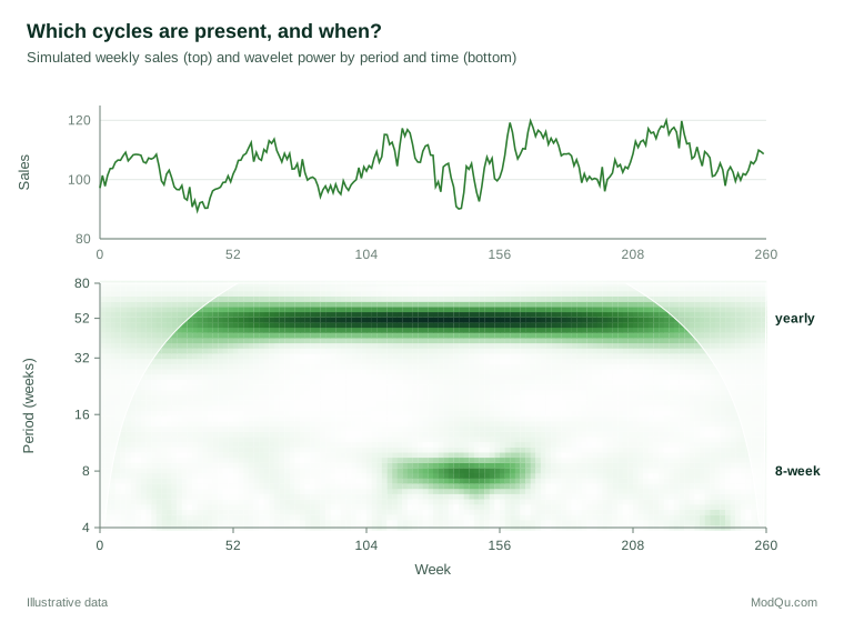
The wavelet power spectrum separates the two clearly. A dark band at a period of 52 weeks runs across the whole series, showing the stable seasonal pattern. A second band at 8 weeks appears only between weeks 110 and 170 and disappears afterwards. A Fourier analysis of the same data would show a peak near 8 weeks, but it could not show that the cycle was present for little more than a year. For the retailer, this places the cycle in time and links it to the promotion schedule that caused it.
Other uses
Denoising. Donoho and Johnstone (1994) showed that removing small wavelet coefficients and keeping large ones, a method called wavelet thresholding or shrinkage, removes noise while keeping sharp features such as sudden jumps, which ordinary smoothing tends to blur. Nason (2008) describes these methods and their software.
Relationships between series. Wavelet coherence measures how strongly two series move together at each scale and time, and the phase shows which one leads. Grinsted et al. (2004) popularised the method in geophysics. In economics, it has been used to study, for example, how the link between interest rates and output changes over time and differs between short and long horizons (Aguiar-Conraria & Soares, 2014). Crowley (2007) gives an introduction aimed at economists.
Survey and market research. For tracking surveys, wavelets can separate long-term shifts in attitudes from short-term reactions to events, and show whether a seasonal pattern in responses is stable or changing. The discrete transform can also split a sales or response series into short-term, medium-term and long-term components, so that each can be modelled or forecast separately and the forecasts added back together. This is useful when different forces drive the series at different horizons, such as weekly promotions and multi-year changes in the market.
Practical guidance
- Choose the wavelet to suit the goal. The Morlet wavelet suits the detection of cycles; compact wavelets such as those of Daubechies suit decomposition and denoising.
- Respect the cone of influence. Do not interpret patterns near the beginning or end of the series.
- Test against a null model. Compare power with what random noise with similar autocorrelation would produce before calling a cycle real.
- Use enough data. A cycle needs to repeat several times within the series to be detected reliably.
Key takeaways
Wavelet analysis shows not only which cycles are present in a time series but when they occur, how strong they are and how they change. The continuous transform produces a time-period map for exploring cycles; the discrete transform splits a series into scale components for decomposition and denoising. Used with care at the edges and with tests against noise, wavelets give researchers a clear view of temporal patterns at several scales at once.
References
Aguiar-Conraria, L., & Soares, M. J. (2014). The continuous wavelet transform: Moving beyond uni- and bivariate analysis. Journal of Economic Surveys, 28(2), 344–375. https://doi.org/10.1111/joes.12012
Crowley, P. M. (2007). A guide to wavelets for economists. Journal of Economic Surveys, 21(2), 207–267. https://doi.org/10.1111/j.1467-6419.2006.00502.x
Daubechies, I. (1992). Ten lectures on wavelets. Society for Industrial and Applied Mathematics. https://doi.org/10.1137/1.9781611970104
Donoho, D. L., & Johnstone, I. M. (1994). Ideal spatial adaptation by wavelet shrinkage. Biometrika, 81(3), 425–455. https://doi.org/10.1093/biomet/81.3.425
Grinsted, A., Moore, J. C., & Jevrejeva, S. (2004). Application of the cross wavelet transform and wavelet coherence to geophysical time series. Nonlinear Processes in Geophysics, 11(5/6), 561–566. https://doi.org/10.5194/npg-11-561-2004
Grossmann, A., & Morlet, J. (1984). Decomposition of Hardy functions into square integrable wavelets of constant shape. SIAM Journal on Mathematical Analysis, 15(4), 723–736. https://doi.org/10.1137/0515056
Mallat, S. G. (1989). A theory for multiresolution signal decomposition: The wavelet representation. IEEE Transactions on Pattern Analysis and Machine Intelligence, 11(7), 674–693. https://doi.org/10.1109/34.192463
Nason, G. P. (2008). Wavelet methods in statistics with R. Springer. https://doi.org/10.1007/978-0-387-75961-6
Percival, D. B., & Walden, A. T. (2000). Wavelet methods for time series analysis. Cambridge University Press. https://doi.org/10.1017/CBO9780511841040
Torrence, C., & Compo, G. P. (1998). A practical guide to wavelet analysis. Bulletin of the American Meteorological Society, 79(1), 61–78. https://doi.org/10.1175/1520-0477(1998)079<0061:APGTWA>2.0.CO;2