
Statistics · Communication and misuse
Regression to the Mean in Business Performance
Why star performers tend to slip and laggards tend to recover, how this statistical effect fools managers into crediting or blaming the wrong causes, and how to analyse performance data without being misled.
A regional manager singles out the ten worst-performing stores of the year for an intensive improvement programme. Twelve months later, nine of the ten have improved, and the programme is declared a success. Meanwhile, the ten best stores, praised and rewarded, mostly did worse. Both stories may have very little to do with the programme or the praise. They are what regression to the mean predicts whenever performance is partly a matter of chance and units are selected because they were extreme.
Regression to the mean is one of the oldest ideas in statistics and one of the most frequently overlooked in management. This article explains what it is, why it happens, how large it can be, and how to design performance reviews, interventions and survey trackers so that it does not masquerade as cause and effect.
Where the idea comes from
Francis Galton first described the effect in the 1880s while studying the heights of parents and their adult children. Unusually tall parents tended to have children who were tall, but on average less extreme than the parents; unusually short parents tended to have children who were somewhat taller than themselves (Galton, 1886). Galton called this "regression towards mediocrity". He initially suspected a biological mechanism, but it was soon understood to be a purely statistical consequence of imperfect correlation between two measurements (Stigler, 1986). The word "regression" in "regression analysis" is inherited from this work.
The business version of the error has a famous history. In 1933, a statistician published a lengthy study showing that firms which were highly profitable at the start of a period became less profitable later, while weak firms improved, and concluded that competition drives businesses toward mediocrity. As Stigler (1997) recounts, the finding was a regression artefact: grouping firms by their initial results guarantees that the groups will converge, even if nothing about competition changes.
Why it happens
Any observed performance figure can be thought of as two parts: a persistent component (skill, location, product mix, management quality) and a transient component (luck, weather, one-off contracts, measurement noise). When we select the units with the highest observed results, we select units that are probably good and probably lucky. Next period, the persistent part tends to stay, but the luck is drawn afresh and is, on average, ordinary. The group's average therefore moves back toward the overall mean.
If two measurements have correlation r and the same mean μ and spread, the expected value of the second measurement given the first is:
E(Y2 | Y1) = μ + r × (Y1 − μ)
When r = 1, performance repeats perfectly and there is no regression. When r = 0, the first result tells us nothing and every unit is expected to return to the mean. Between these extremes, a unit is expected to keep a fraction r of its distance from the average, and lose the rest. Barnett et al. (2005) give formulas for the expected size of the effect when units are selected above or below a cut-off, and show that it grows as the correlation falls and as the selection becomes more extreme.
Two points are worth stressing. First, regression to the mean is a property of groups selected on an extreme measurement, not a force that pulls individuals toward the middle. The overall spread of performance need not shrink from one year to the next, because new units become extreme by chance as others return. Second, the effect runs in both directions in time: the best performers this year were, on average, less exceptional last year too (Bland & Altman, 1994).
A worked example
Consider a hypothetical retailer with 200 stores. Year-on-year sales growth averages 4% with a standard deviation of 3 percentage points, and the correlation between a store's growth in one year and the next is 0.5. Half of the variation between stores is persistent and half is transient.
Rank the stores on year 1 and divide them into five equal groups. Applying the formula above gives the expected year 2 growth for each group (Figure 1). The top fifth averaged 8.2% in year 1; the same stores are expected to average 6.1% in year 2. The bottom fifth averaged −0.2% and is expected to recover to 1.9%. No store has changed anything.
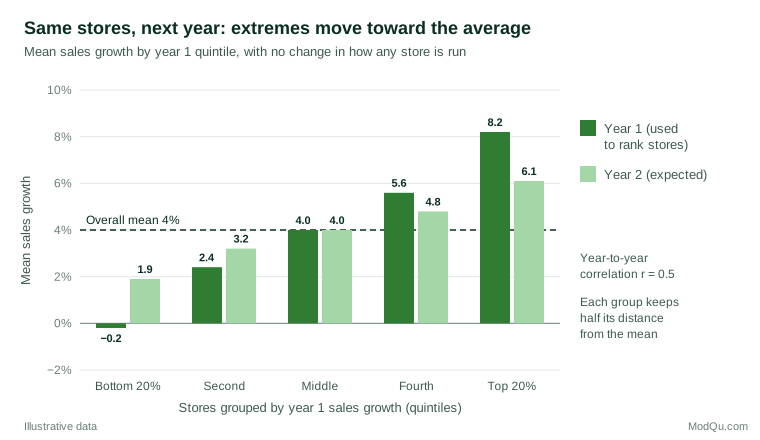
Now imagine the retailer had put the bottom fifth through a training programme. It would report an improvement of 2.1 points and might attribute it to the training. The true effect of the programme could be zero. Equally, a bonus scheme for the top fifth might appear to "cause complacency", since those stores' growth fell by 2.1 points.
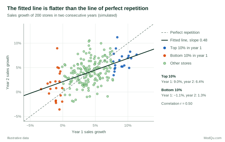
Figure 2 shows a simulated version of the same situation for individual stores. The dashed line marks where stores would sit if performance repeated exactly. The fitted line is much flatter, with a slope close to the correlation of 0.5. The stores in the top tenth in year 1 averaged 9.0% growth but only 6.4% in year 2, while the bottom tenth rose from −1.1% to 1.3%.
Where it misleads business decisions
Praise, punishment and coaching. Tversky and Kahneman (1974) describe flight instructors who concluded that praise for a smooth landing made the next landing worse, while criticism of a rough landing improved it. The pattern was regression to the mean: exceptional landings, good or bad, were usually followed by more typical ones. Sales managers who reward the month's top performer and reprimand the bottom one will see the same pattern and may draw the same false lesson.
Turnaround programmes and interventions. Any intervention aimed at units chosen because they performed badly will look effective. Campbell (1969) analysed a crackdown on speeding introduced after a year of record traffic deaths in Connecticut and showed that much of the subsequent fall could be expected from regression alone. Morton and Torgerson (2003) make the same point for health care, where road safety cameras and treatment programmes are often placed where recent results were worst. Business equivalents include "special measures" for failing branches, coaching for low-scoring call-centre agents and remedial campaigns in regions with a bad quarter.
Celebrated companies and managers. Firms profiled as exemplars are usually chosen at a peak. Rosenzweig (2007) argues that many companies held up as models of excellence later performed quite ordinarily, and that business writers often attribute to strategy and culture what was partly good fortune. Studies of corporate earnings find that unusually high or low profitability tends to revert toward the average over a few years (Fama & French, 2000).
Choosing the best option. When managers select the project, supplier or campaign with the highest estimated return, they systematically select estimates that were too high. Smith and Winkler (2006) call this the optimiser's curse and show that the chosen option will, on average, disappoint. The same logic explains why the winning variant of an online experiment often shows a smaller lift when rolled out; Kohavi et al. (2020) advise treating surprisingly large results with suspicion and replicating them.
League tables and rankings. Small units, such as branches with few customers or survey cells with few respondents, produce more variable results and therefore dominate both ends of any ranking. Wainer (2007) shows how this led to mistaken enthusiasm for small schools. Goldstein and Spiegelhalter (1996) warn that rankings of institutions ignore this uncertainty, and much of the movement between one year's table and the next is regression to the mean.
How large is the effect?
The size of the effect depends on two things: how reliable the measure is and how extreme the selection is. Customer satisfaction scores from a few dozen responses per branch, monthly sales for small accounts and individual employee ratings are noisy, so their year-to-year correlations may be low and regression large. Annual revenue of large stores is more stable and regresses less. A simple check is to compute the correlation between two consecutive periods for the units in question. If it is 0.3, an extreme group is expected to keep only about 30% of its advantage; if it is 0.9, about 90%.
People rarely make this adjustment intuitively. Kahneman and Tversky (1973) found that predictions are typically not regressive enough: people predict that an extreme performer will stay as extreme as the evidence appears, even when they know the evidence is unreliable.
Practical guidance
- Use a control group. The most reliable defence is to compare treated units with similar units, selected in the same way, that did not receive the intervention. Random allocation among the low performers is best, because both groups then regress by the same expected amount (Barnett et al., 2005).
- Do not select and evaluate on the same measurement. If branches are chosen on one quarter's results, judge improvement against a separate baseline, such as an average of several earlier periods. Averaging several measurements reduces the transient component (Barnett et al., 2005).
- Estimate the expected regression. Use the correlation between periods to predict where selected units would have landed anyway, and compare the actual result with that prediction rather than with their starting point (Campbell & Kenny, 1999).
- Shrink extreme estimates. Methods that pull noisy unit-level estimates toward the overall mean, such as empirical Bayes or multilevel models, give better predictions of future performance than the raw figures. Efron and Morris (1977) showed this with baseball batting averages, and Efron and Hastie (2016) explain the general principle.
- Show uncertainty in rankings. Funnel plots, which plot each unit's result against its size with control limits, show which units are genuinely unusual and which are merely small (Spiegelhalter, 2005).
- Be wary of "most improved" and "biggest decline" lists. These are often lists of units that were unlucky or lucky in the previous period.
Common mistakes
- Inventing causes for change. Explaining every rise and fall with a story about leadership, morale or strategy, when much of it is noise.
- Ignoring selection. Reporting that "the stores we targeted improved by 2 points" without stating that they were chosen because they had just done badly.
- Assuming the effect is small in large samples. Regression depends on the correlation between periods, not on the total number of units. A dataset of 10,000 branches can show large regression if each branch's result is noisy.
- Overcorrecting. Not every improvement is regression. If a control group improves by 2 points and the treated group by 5, the extra 3 points may be a real effect.
Key takeaways
Whenever performance is measured with error or influenced by luck, units selected for being extreme will tend to look more ordinary next time. This is regression to the mean, and it can make useless interventions look effective, make praise look harmful and turn yesterday's stars into today's disappointments. The remedies are statistical rather than managerial: compare with a control group, avoid selecting and evaluating on the same data, estimate how much regression to expect, shrink noisy estimates and show uncertainty in rankings. Managers who understand the effect make fairer judgements of people and more accurate judgements of programmes.
References
Barnett, A. G., van der Pols, J. C., & Dobson, A. J. (2005). Regression to the mean: What it is and how to deal with it. International Journal of Epidemiology, 34(1), 215–220. https://doi.org/10.1093/ije/dyh299
Bland, J. M., & Altman, D. G. (1994). Regression towards the mean. BMJ, 308(6942), 1499. https://doi.org/10.1136/bmj.308.6942.1499
Campbell, D. T. (1969). Reforms as experiments. American Psychologist, 24(4), 409–429. https://doi.org/10.1037/h0027982
Campbell, D. T., & Kenny, D. A. (1999). A primer on regression artifacts. Guilford Press.
Efron, B., & Hastie, T. (2016). Computer age statistical inference: Algorithms, evidence, and data science. Cambridge University Press. https://doi.org/10.1017/CBO9781316576533
Efron, B., & Morris, C. (1977). Stein's paradox in statistics. Scientific American, 236(5), 119–127. https://doi.org/10.1038/scientificamerican0577-119
Fama, E. F., & French, K. R. (2000). Forecasting profitability and earnings. The Journal of Business, 73(2), 161–175. https://doi.org/10.1086/209638
Galton, F. (1886). Regression towards mediocrity in hereditary stature. The Journal of the Anthropological Institute of Great Britain and Ireland, 15, 246–263. https://doi.org/10.2307/2841583
Goldstein, H., & Spiegelhalter, D. J. (1996). League tables and their limitations: Statistical issues in comparisons of institutional performance. Journal of the Royal Statistical Society Series A: Statistics in Society, 159(3), 385–443. https://doi.org/10.2307/2983325
Kahneman, D., & Tversky, A. (1973). On the psychology of prediction. Psychological Review, 80(4), 237–251. https://doi.org/10.1037/h0034747
Kohavi, R., Tang, D., & Xu, Y. (2020). Trustworthy online controlled experiments: A practical guide to A/B testing. Cambridge University Press. https://doi.org/10.1017/9781108653985
Morton, V., & Torgerson, D. J. (2003). Effect of regression to the mean on decision making in health care. BMJ, 326(7398), 1083–1084. https://doi.org/10.1136/bmj.326.7398.1083
Rosenzweig, P. (2007). The halo effect: And the eight other business delusions that deceive managers. Free Press.
Smith, J. E., & Winkler, R. L. (2006). The optimizer's curse: Skepticism and postdecision surprise in decision analysis. Management Science, 52(3), 311–322. https://doi.org/10.1287/mnsc.1050.0451
Spiegelhalter, D. J. (2005). Funnel plots for comparing institutional performance. Statistics in Medicine, 24(8), 1185–1202. https://doi.org/10.1002/sim.1970
Stigler, S. M. (1986). The history of statistics: The measurement of uncertainty before 1900. Belknap Press of Harvard University Press.
Stigler, S. M. (1997). Regression towards the mean, historically considered. Statistical Methods in Medical Research, 6(2), 103–114. https://doi.org/10.1177/096228029700600202
Tversky, A., & Kahneman, D. (1974). Judgment under uncertainty: Heuristics and biases. Science, 185(4157), 1124–1131. https://doi.org/10.1126/science.185.4157.1124
Wainer, H. (2007). The most dangerous equation. American Scientist, 95(3), 249. https://doi.org/10.1511/2007.65.1026