
Statistics · Communication and misuse
Simpson's Paradox: When Aggregated Data Mislead
Why a comparison that holds in every subgroup can reverse when the groups are combined, shown with the kidney stone data and a business experiment, and how to decide which figure to trust.
A treatment that works better for every type of patient can still look worse overall. A website change that lifts conversion on every day of a test can still appear to lower it across the whole test. These reversals are not arithmetic errors but examples of Simpson's paradox, a major trap in the reporting of rates, percentages and averages. Anyone who reads totals from a dashboard, a cross-tabulation or a survey report needs to know when the total can be trusted and when it cannot.
What the paradox is
Simpson's paradox occurs when an association between two variables, seen within each level of a third variable, weakens, disappears or reverses when the levels are combined. Yule (1903) noted the possibility in his work on the association of attributes, and Simpson (1951) gave the formal treatment that gave the paradox its name. Blyth (1972) showed how sharply it can conflict with intuition: an option can be better in every subgroup yet worse in the aggregate, which seems to break the common-sense rule that something better in every case should be better overall.
The mathematics is sound. An overall rate is a weighted average of subgroup rates, and the weights are the shares of each group in the total. When two options are compared, each has its own weights. If one option is concentrated in a subgroup where outcomes are poor for everyone, its overall rate is pulled down, however well it performs within that subgroup.
A classic example: kidney stone treatments
Charig et al. (1986) compared treatments for kidney stones. Julious and Mullee (1994) used two of them, open surgery and percutaneous nephrolithotomy, to illustrate the paradox. The table shows the numbers of successful treatments.
| Stone size | Open surgery | Percutaneous nephrolithotomy |
|---|---|---|
| Small stones | 81 of 87 (93%) | 234 of 270 (87%) |
| Large stones | 192 of 263 (73%) | 55 of 80 (69%) |
| All patients | 273 of 350 (78%) | 289 of 350 (83%) |
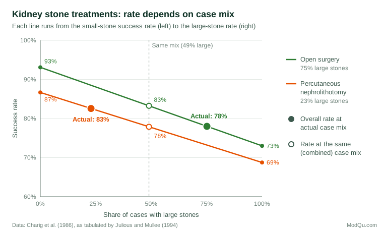
Open surgery had the higher success rate for small stones and for large stones. Yet across all 350 patients in each group, percutaneous nephrolithotomy appeared better, by 83% to 78%. The explanation lies in who received which treatment. Large stones are harder to treat, and clinicians more often chose open surgery for them: 75% of open surgery patients had large stones, against 23% of those treated percutaneously. Stone size was associated with both the choice of treatment and the outcome, which makes it a confounder of the comparison (Julious & Mullee, 1994).
Figure 1 shows the mechanism. Each line runs from a treatment's success rate for small stones to its rate for large stones, and every point on the line is the overall rate that the treatment would achieve with a given mix of cases. Open surgery's line lies above the other line everywhere. The overall rates differ only because the two treatments sit at very different points on the horizontal axis.
Putting the groups on an equal footing
The simplest correction is standardisation: apply each treatment's subgroup rates to the same case mix. In the combined data, 51% of patients had small stones and 49% had large stones.
Standardised rate = Σ wk × pk
where wk is the share of subgroup k in a common reference population and pk is the option's rate in that subgroup. With the common weights, open surgery's success rate is 0.51 × 93.1% + 0.49 × 73.0% ≈ 83.3%, and percutaneous nephrolithotomy's is 0.51 × 86.7% + 0.49 × 68.8% ≈ 77.9%. The ranking reverses back, matching the within-group comparisons. The same idea underlies the Mantel–Haenszel estimator, which pools the odds ratios across strata (Mantel & Haenszel, 1959). For these data it gives a pooled odds ratio of about 1.45 in favour of open surgery, whereas the crude odds ratio from the totals is about 0.75 and points the other way.
A business example: an experiment that changed its traffic split
The paradox is common in online experiments when the share of traffic sent to a new version changes during the test. Kohavi et al. (2020) describe how ramping up a test, for example from a small share of users on the first day to an even split later, can produce misleading combined results. Consider a hypothetical checkout test run over a Friday and a Saturday. Friday shoppers convert far more often than Saturday browsers, and the new design received only 10% of Friday's traffic but half of Saturday's.
| Day | Current design | New design |
|---|---|---|
| Friday | 2,700 of 90,000 (3.0%) | 320 of 10,000 (3.2%) |
| Saturday | 500 of 50,000 (1.0%) | 550 of 50,000 (1.1%) |
| Both days | 3,200 of 140,000 (2.3%) | 870 of 60,000 (1.45%) |
The new design converts better on each day, but its pooled rate is much lower, because most of its visitors arrived on the low-converting day. The correct analysis compares the designs within each day, or weights the days equally for both designs. Similar reversals appear in sales comparisons across regions, satisfaction scores across branches and public statistics. Wagner (1982) collected real cases, including United States income tax figures in which the average tax rate fell within each income bracket while the overall rate rose, because rising incomes moved more taxpayers into higher brackets.
Which answer is right?
It is tempting to conclude that the disaggregated figures are always correct. They are not. Whether to combine or separate the groups depends on the causal relationships among the variables, not on the numbers in the table (Pearl, 2009). Pearl (2014) argues that the paradox only seems puzzling because people read the data causally without stating the causal story, and that once the story is explicit the right choice follows.
- If the grouping variable is a confounder, a cause of both the choice and the outcome, the subgroup comparison (or a standardised one) is appropriate. Stone size existed before treatment and influenced which treatment was chosen, so the kidney stone comparison should be made within stone size.
- If the grouping variable lies on the causal path, a result of the option being compared, splitting by it can hide the very effect of interest. If a drug lowers blood pressure and thereby improves survival, comparing survival within blood pressure levels removes part of the drug's benefit. Here the aggregate comparison answers the question of the total effect.
- If the grouping variable is affected by both the option and the outcome, conditioning on it can create a spurious association. This is collider bias (Elwert & Winship, 2014).
Hernán et al. (2011) show that the same table of numbers can call for different analyses depending on which of these structures applies. The paradox therefore cannot be resolved by statistics alone. It needs knowledge of how the data came about, ideally set out in a causal diagram (Greenland et al., 1999).
Detecting and handling the paradox in practice
- Break totals down by the main segments. When groups being compared differ in composition, look at the rates within segments such as region, customer type, channel or time period before reporting the total.
- Compare compositions, not only rates. A quick check of the mix in each group, such as the share of large stones or of Saturday traffic, shows whether a reversal is possible.
- Standardise or model. Use direct standardisation, stratified estimators or regression with the relevant covariates when a fair comparison needs a common mix. Kievit et al. (2013) give a practical guide, including visual checks for spotting reversals.
- Design it out. Randomisation balances confounders on average, and a constant allocation ratio in experiments prevents ramp-up reversals (Kohavi et al., 2020).
- Remember the reverse problem. Group-level relationships do not necessarily hold for individuals either. Robinson (1950) showed that correlations across areas can differ greatly from those across the people who live in them, the ecological fallacy.
Common mistakes
- Reporting a single pooled rate for groups that differ markedly in composition, such as new and established stores.
- Adjusting for everything available. Adding a variable that is a consequence of the option, or a collider, can introduce the bias it was meant to remove.
- Assuming that more detail is always better. Very fine subgroups have small samples, and apparent reversals can then be noise.
- Changing the mix over time in trackers and experiments, then comparing totals across waves.
Key takeaways
Simpson's paradox is a reminder that an overall rate mixes two things: how well each option performs within groups and how its cases are spread across those groups. When groups differ in composition, aggregate figures can point in the opposite direction from every subgroup. Check compositions, compare like with like through stratification or standardisation, and decide which comparison answers the question by thinking through the causal structure, not by choosing the figure that tells the more convenient story.
References
Blyth, C. R. (1972). On Simpson's paradox and the sure-thing principle. Journal of the American Statistical Association, 67(338), 364–366. https://doi.org/10.1080/01621459.1972.10482387
Charig, C. R., Webb, D. R., Payne, S. R., & Wickham, J. E. A. (1986). Comparison of treatment of renal calculi by open surgery, percutaneous nephrolithotomy, and extracorporeal shockwave lithotripsy. BMJ, 292(6524), 879–882. https://doi.org/10.1136/bmj.292.6524.879
Elwert, F., & Winship, C. (2014). Endogenous selection bias: The problem of conditioning on a collider variable. Annual Review of Sociology, 40, 31–53. https://doi.org/10.1146/annurev-soc-071913-043455
Greenland, S., Pearl, J., & Robins, J. M. (1999). Causal diagrams for epidemiologic research. Epidemiology, 10(1), 37–48. https://doi.org/10.1097/00001648-199901000-00008
Hernán, M. A., Clayton, D., & Keiding, N. (2011). The Simpson's paradox unraveled. International Journal of Epidemiology, 40(3), 780–785. https://doi.org/10.1093/ije/dyr041
Julious, S. A., & Mullee, M. A. (1994). Confounding and Simpson's paradox. BMJ, 309(6967), 1480–1481. https://doi.org/10.1136/bmj.309.6967.1480
Kievit, R. A., Frankenhuis, W. E., Waldorp, L. J., & Borsboom, D. (2013). Simpson's paradox in psychological science: A practical guide. Frontiers in Psychology, 4, 513. https://doi.org/10.3389/fpsyg.2013.00513
Kohavi, R., Tang, D., & Xu, Y. (2020). Trustworthy online controlled experiments: A practical guide to A/B testing. Cambridge University Press. https://doi.org/10.1017/9781108653985
Mantel, N., & Haenszel, W. (1959). Statistical aspects of the analysis of data from retrospective studies of disease. Journal of the National Cancer Institute, 22(4), 719–748. https://doi.org/10.1093/jnci/22.4.719
Pearl, J. (2009). Causality: Models, reasoning, and inference (2nd ed.). Cambridge University Press. https://doi.org/10.1017/CBO9780511803161
Pearl, J. (2014). Comment: Understanding Simpson's paradox. The American Statistician, 68(1), 8–13. https://doi.org/10.1080/00031305.2014.876829
Robinson, W. S. (1950). Ecological correlations and the behavior of individuals. American Sociological Review, 15(3), 351–357. https://doi.org/10.2307/2087176
Simpson, E. H. (1951). The interpretation of interaction in contingency tables. Journal of the Royal Statistical Society Series B: Statistical Methodology, 13(2), 238–241. https://doi.org/10.1111/j.2517-6161.1951.tb00088.x
Wagner, C. H. (1982). Simpson's paradox in real life. The American Statistician, 36(1), 46–48. https://doi.org/10.1080/00031305.1982.10482778
Yule, G. U. (1903). Notes on the theory of association of attributes in statistics. Biometrika, 2(2), 121–134. https://doi.org/10.1093/biomet/2.2.121