
Statistics · Communication and misuse
How to Lie With Statistics: Common Distortions and How to Spot Them
A practical guide to the classic ways numbers mislead, from well-chosen averages and relative risks to biased samples, selective reporting and distorted charts, with questions any reader can ask.
In 1954 the journalist Darrell Huff published a small, cheerful book called How to Lie with Statistics. It explained, with cartoons, how averages could be chosen to flatter, how samples could be built to give the desired answer, and how charts could turn a modest change into a dramatic one (Huff, 1954). Seventy years later the techniques are unchanged, but far more numbers reach managers and customers, usually without any explanation of how they were produced.
Most misleading statistics are not deliberate lies. They arise from choices that each seem reasonable: which average to report, which baseline to compare against, which subgroup to highlight, which axis to draw. Best (2001) calls the results "mutant statistics": figures that began as honest estimates but were simplified, repeated and stretched until they no longer meant what their authors intended. This article describes the most common distortions, why each works, and questions for spotting them. Anyone who commissions, analyses or presents survey and market research should know these patterns well enough to avoid them.
1. The well-chosen average
"The average customer spends $659 a year" sounds like a description of a typical customer. It may not be. When a distribution is skewed, as spending, income, order values and company sizes usually are, the mean is pulled toward the long tail by a small number of very large values, while the median marks the middle customer.
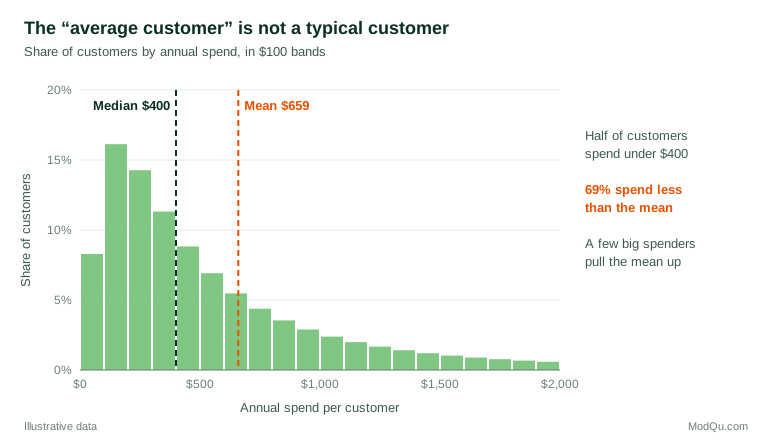
Both figures in Figure 1 are correct. The mean suits forecasting total revenue; the median better describes an ordinary customer. The distortion lies in choosing whichever one supports the argument and calling it "the average" without saying which. Huff (1954) called this the "well-chosen average".
How to spot it: ask which average is meant, and whether the distribution is skewed. If the report gives only a mean for something like income, spending or time on site, ask for the median as well.
2. Relative risk without the baseline
Suppose a change to the order process cuts complaints from 4 per 100 orders to 2 per 100. A press release can say "complaints halved". An internal note can say "two fewer complaints per 100 orders". Both are true (Figure 2). The first is a relative change and the second is an absolute change, and they create very different impressions.
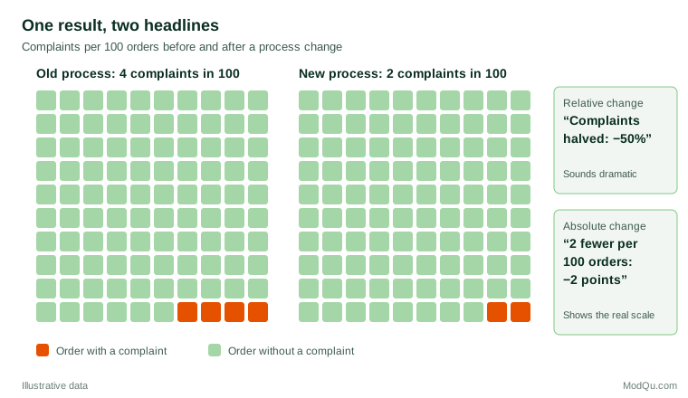
Relative figures are especially persuasive when the baseline is small. Gigerenzer et al. (2007) document how health benefits are routinely reported as relative risk reductions. For example, a screening programme that reduces deaths from 4 to 3 in every 1,000 people can be described as a "25% reduction", while the absolute reduction is one person in 1,000. Their review shows that both patients and doctors overestimate benefits when given only relative figures, and that natural frequencies and absolute numbers are much easier to understand. Spiegelhalter (2017) makes the same recommendation for risk communication generally: give the baseline, use frequencies with a common denominator, and present absolute changes alongside relative ones.
A related confusion is between percent and percentage points. A conversion rate that rises from 2% to 3% has increased by one percentage point, or by 50%. Reports that say "conversion up 50%" without the starting rate leave readers unable to judge whether the change matters.
How to spot it: whenever a change is expressed as a percentage, ask "a percentage of what?" and look for the starting level.
3. The sample with the built-in bias
The most famous polling failure in history is a lesson in sample bias. In 1936 the Literary Digest magazine mailed ballots to millions of Americans and received more than two million replies, which pointed to a clear defeat for President Roosevelt. Roosevelt won by a landslide. Squire (1988), using survey data collected the following year, concluded that the magazine's lists of names leaned toward wealthier voters and, more importantly, that those who chose to return the ballot differed from those who did not. Size did not rescue a biased sample.
The modern equivalents are opt-in web polls, website feedback widgets and customer reviews. People who respond voluntarily are often those with strong opinions, more time or more interest. Bethlehem (2010) shows that self-selection in web surveys can produce bias that does not shrink as the sample grows. Meng (2018) quantified the point dramatically: a large non-random sample with even a tiny correlation between who is included and what is measured can carry no more information than a small random sample. When a claim rests on "50,000 responses", the number of responses is less important than how respondents came to be included.
How to spot it: ask who was asked, who answered, and who was left out. A nonprobability sample is not necessarily useless, but its results need weighting, comparison with known benchmarks and careful wording about whom they represent.
4. Questions that write the answer
Survey results can be shaped before a single respondent is contacted. The wording of a question, the response options offered and the order of questions all influence answers. Schwarz (1999) reviews experimental evidence showing that respondents use every feature of a questionnaire, including the numeric labels on a rating scale and the range of response categories, to work out what the question means, so that small design changes can shift reported behaviours and opinions considerably.
Framing works in a similar way. Tversky and Kahneman (1981) showed that people's choices between identical options reversed depending on whether outcomes were described as lives saved or lives lost. In business research, a question that asks whether customers "would welcome a modest price adjustment to support improved service" will produce a different result from one that asks whether they "would accept a price rise". Leading questions and unbalanced scales bias results toward the sponsor's preferred answer.
How to spot it: ask to see the exact question wording and response options. Reputable research organisations publish them alongside the results.
5. The little figures that are not there
Some distortions work by omission. A claim that "satisfaction rose to 82%" means little without the sample size, the margin of error, the previous figure and the date. A subgroup of 40 respondents can swing by many points through sampling error alone. Huff (1954) called these "the little figures that are not there", and the list of missing figures is long:
- the base, or number of cases, behind a percentage;
- the margin of error or confidence interval;
- the comparison group or previous period;
- the time period chosen and why;
- the share of people who did not respond, or who answered "don't know".
Statistical significance is also often used to make small differences look important. A statistically significant result is not necessarily large or useful, and a non-significant result does not show that there is no effect. The American Statistical Association's statement on p-values stresses that a p-value does not measure the size of an effect or the importance of a result (Wasserstein & Lazar, 2016).
How to spot it: look for the base sizes, intervals and comparison points. If they are missing, ask for them before relying on the figure.
6. Correlation presented as causation
A strong association between two variables does not show that one causes the other. Huff (1954) called this the "post hoc" fallacy. Messerli (2012) memorably reported a strong correlation (r = 0.79) across countries between chocolate consumption per person and the number of Nobel laureates per head of population. The relationship is real in the data, but national wealth, education systems and many other factors could explain it, and nobody seriously suggests that chocolate wins prizes.
Business examples are more tempting. Customers who use a loyalty app spend more, but loyal customers were always more likely to download it. Without a controlled experiment or a careful causal design, such patterns may reflect confounding or reverse causation rather than the effect claimed.
How to spot it: ask whether the claim is about association or about cause, and what else could explain the pattern.
7. Aggregation that reverses the story
Combining groups can produce a result that holds in none of them. In a well-known analysis of graduate admissions at the University of California, Berkeley, the overall figures suggested that men were admitted at a higher rate than women. When Bickel et al. (1975) examined individual departments, most showed no bias against women, and some showed a small advantage for them. Women had applied disproportionately to departments with low admission rates for everyone. This reversal, known as Simpson's paradox, can occur whenever groups differ in size and composition.
In market research, a company-wide satisfaction score can change only because the mix of customer types has shifted.
How to spot it: ask whether the overall figure holds within the main subgroups, and whether the composition of the groups has changed.
8. Selective reporting and the garden of analyses
When analysts test many outcomes, subgroups and time windows, some will show "significant" results by chance. Reporting only those, without saying how many were tried, produces findings that are unlikely to be repeated. Simmons et al. (2011) showed that a few common and individually defensible choices, such as testing several measures or stopping data collection when a result looked good, could make the chance of a false positive far higher than the nominal 5%. Kerr (1998) described the related practice of presenting a hypothesis developed after seeing the results as if it had been stated in advance, known as HARKing.
Selection also happens at the level of whole studies. Rosenthal (1979) named the file-drawer problem: studies with null results are less likely to be published, so the visible literature overstates effects. Ioannidis (2005) argued that when studies are small, effects are modest, many relationships are tested and flexibility is high, most claimed research findings may be false. Commercial analyses can likewise be rerun until they deliver a welcome answer.
How to spot it: ask how many comparisons were made, whether the hypotheses and outcome measures were set in advance, and whether results that did not support the conclusion are also reported.
9. Pictures that exaggerate
Charts are powerful because readers take in their message before checking the numbers. A bar chart whose vertical axis starts at 95% instead of zero can make a difference of two points look like a doubling. A pictogram that scales an icon in both height and width makes a twofold increase look fourfold. Tufte (2001) proposed the lie factor, the size of an effect shown in a graphic divided by the size of the effect in the data, as a simple measure of such exaggeration. Wainer (1984) catalogued many ways of "displaying data badly", from hiding the data to emphasising the trivial.
These effects are not merely theoretical. In experiments by Pandey et al. (2015), truncated axes, distorted areas and inverted axes all changed how participants judged the messages of charts, even when the correct numbers were printed on them. Graph-specific distortions, including truncated axes, cherry-picked time ranges and dual axes, are discussed in detail in a separate ModQu article.
How to spot it: read the axis labels and scales before the shape. Check where the axis starts, whether the time range has been chosen to tell a particular story, and whether area or volume is being used to show a single quantity.
10. Numbers that become targets
Finally, statistics can be distorted by the people being measured. Campbell (1979) observed that the more a quantitative indicator is used for social decision-making, the more it is subject to corruption pressures, and the more it distorts the processes it is meant to monitor. Businesses see this when agents end calls quickly to meet handling-time targets or staff coach customers to give top satisfaction scores. The number improves while the thing it was meant to measure does not.
How to spot it: ask whether the people producing the figure are rewarded on it, and whether other indicators tell the same story.
A checklist for any statistic
Huff (1954) ended his book with five questions: who says so, how do they know, what is missing, did somebody change the subject, and does it make sense? Best (2001) and Spiegelhalter (2019) offer similar lists. Gal (2002) argues that statistical literacy for adults requires not only knowledge of statistics but also a critical disposition: the habit of asking questions about numbers rather than accepting them. A practical version for business readers is:
- Source and motive. Who produced the number, who paid for it, and what do they want readers to conclude?
- Definition. What exactly is being counted or measured, and has the definition changed over time?
- Sample. Who was included, how were they selected, and how many were there?
- Measurement. What question was asked, and how might the wording or format have influenced the answer?
- Comparison. Compared with what? Is the baseline, previous period or control group shown?
- Size and uncertainty. Is the effect large enough to matter, and how precise is the estimate?
- Alternative explanations. Could chance, selection, confounding or a change in mix explain the result?
- Presentation. Do the chart and headline match the numbers underneath?
Practical guidance for researchers and report writers
The same list is a standard for honest reporting. Give base sizes, intervals, fieldwork dates, sample source, question wording and weighting. Report absolute and relative changes together, use medians for skewed measures, start bar-chart axes at zero, and label unplanned comparisons as exploratory.
Key takeaways
Statistics rarely lie on their own. They mislead through flattering averages, relative changes without baselines, self-selected samples, loaded wording, missing uncertainty, correlation sold as cause, aggregation, selective reporting, exaggerated charts and gamed measures. A short set of questions about source, definition, sample, measurement, comparison, size, alternatives and presentation catches most of these problems. Ask them of your own numbers as well as other people's.
References
Best, J. (2001). Damned lies and statistics: Untangling numbers from the media, politicians, and activists. University of California Press.
Bethlehem, J. (2010). Selection bias in web surveys. International Statistical Review, 78(2), 161–188. https://doi.org/10.1111/j.1751-5823.2010.00112.x
Bickel, P. J., Hammel, E. A., & O'Connell, J. W. (1975). Sex bias in graduate admissions: Data from Berkeley. Science, 187(4175), 398–404. https://doi.org/10.1126/science.187.4175.398
Campbell, D. T. (1979). Assessing the impact of planned social change. Evaluation and Program Planning, 2(1), 67–90. https://doi.org/10.1016/0149-7189(79)90048-X
Gal, I. (2002). Adults' statistical literacy: Meanings, components, responsibilities. International Statistical Review, 70(1), 1–25. https://doi.org/10.1111/j.1751-5823.2002.tb00336.x
Gigerenzer, G., Gaissmaier, W., Kurz-Milcke, E., Schwartz, L. M., & Woloshin, S. (2007). Helping doctors and patients make sense of health statistics. Psychological Science in the Public Interest, 8(2), 53–96. https://doi.org/10.1111/j.1539-6053.2008.00033.x
Huff, D. (1954). How to lie with statistics. W. W. Norton.
Ioannidis, J. P. A. (2005). Why most published research findings are false. PLoS Medicine, 2(8), Article e124. https://doi.org/10.1371/journal.pmed.0020124
Kerr, N. L. (1998). HARKing: Hypothesizing after the results are known. Personality and Social Psychology Review, 2(3), 196–217. https://doi.org/10.1207/s15327957pspr0203_4
Meng, X.-L. (2018). Statistical paradises and paradoxes in big data (I): Law of large populations, big data paradox, and the 2016 US presidential election. The Annals of Applied Statistics, 12(2), 685–726. https://doi.org/10.1214/18-AOAS1161SF
Messerli, F. H. (2012). Chocolate consumption, cognitive function, and Nobel laureates. New England Journal of Medicine, 367(16), 1562–1564. https://doi.org/10.1056/NEJMon1211064
Pandey, A. V., Rall, K., Satterthwaite, M. L., Nov, O., & Bertini, E. (2015). How deceptive are deceptive visualizations? An empirical analysis of common distortion techniques. In Proceedings of the 33rd Annual ACM Conference on Human Factors in Computing Systems (pp. 1469–1478). ACM. https://doi.org/10.1145/2702123.2702608
Rosenthal, R. (1979). The file drawer problem and tolerance for null results. Psychological Bulletin, 86(3), 638–641. https://doi.org/10.1037/0033-2909.86.3.638
Schwarz, N. (1999). Self-reports: How the questions shape the answers. American Psychologist, 54(2), 93–105. https://doi.org/10.1037/0003-066X.54.2.93
Simmons, J. P., Nelson, L. D., & Simonsohn, U. (2011). False-positive psychology: Undisclosed flexibility in data collection and analysis allows presenting anything as significant. Psychological Science, 22(11), 1359–1366. https://doi.org/10.1177/0956797611417632
Spiegelhalter, D. (2017). Risk and uncertainty communication. Annual Review of Statistics and Its Application, 4(1), 31–60. https://doi.org/10.1146/annurev-statistics-010814-020148
Spiegelhalter, D. (2019). The art of statistics: Learning from data. Pelican Books.
Squire, P. (1988). Why the 1936 Literary Digest poll failed. Public Opinion Quarterly, 52(1), 125–133. https://doi.org/10.1086/269085
Tufte, E. R. (2001). The visual display of quantitative information (2nd ed.). Graphics Press.
Tversky, A., & Kahneman, D. (1981). The framing of decisions and the psychology of choice. Science, 211(4481), 453–458. https://doi.org/10.1126/science.7455683
Wainer, H. (1984). How to display data badly. The American Statistician, 38(2), 137–147. https://doi.org/10.1080/00031305.1984.10483186
Wasserstein, R. L., & Lazar, N. A. (2016). The ASA statement on p-values: Context, process, and purpose. The American Statistician, 70(2), 129–133. https://doi.org/10.1080/00031305.2016.1154108