
Statistics · Communication and misuse
Survivorship Bias in Data and Decisions
How looking only at the cases that survived a selection process distorts averages, trends and lessons, with examples from aircraft, investment funds, customer cohorts and surveys, and practical checks against it.
During the Second World War, analysts studied the damage on bombers returning from missions. The tempting conclusion was to add armour where the returning aircraft showed the most bullet holes. The statistician Abraham Wald saw the flaw: the aircraft that were hit in other places had not come back to be counted. Damage on the survivors showed where an aircraft could be hit and still return. The story has become the standard illustration of survivorship bias, the error of drawing conclusions from the cases that passed through a selection process while forgetting those that did not.
What survivorship bias is
Survivorship bias is a form of selection bias. A dataset contains only units that "survived" some filter: firms still trading, funds still open, customers still active, respondents still in a panel, products still on sale. If survival is related to the outcome being studied, any average, comparison or trend calculated from the survivors will differ systematically from the truth for the whole original population.
Heckman (1979) showed that analysing a selected sample as if it were random is a specification error, because the selection acts like an omitted variable. Hernán et al. (2004) gave a structural account: selection bias arises when the analysis is restricted to units that share a common effect of the exposure and the outcome. Conditioning on that common effect, a collider, can create associations that do not exist in the full population (Elwert & Winship, 2014). Survival is often exactly such a common effect.
Wald's aircraft, done properly
The popular version of Wald's story is simplified. Mangel and Samaniego (1984) reconstructed his wartime memoranda, which developed a formal method for estimating how vulnerable different parts of an aircraft were from the pattern of damage on those that returned. The key step was to model the hits that were not observed. If hits are spread roughly evenly over an aircraft in combat, then sections with few holes among returning aircraft are sections where hits were most often fatal. The lesson is general. The missing cases do not have to be ignored; with a model of how they went missing, the observed data can still be informative. Wald's approach also shows that an absence among survivors is itself evidence: a pattern that never appears in the surviving cases may be the pattern that was most often fatal.
Investment funds: the disappearing losers
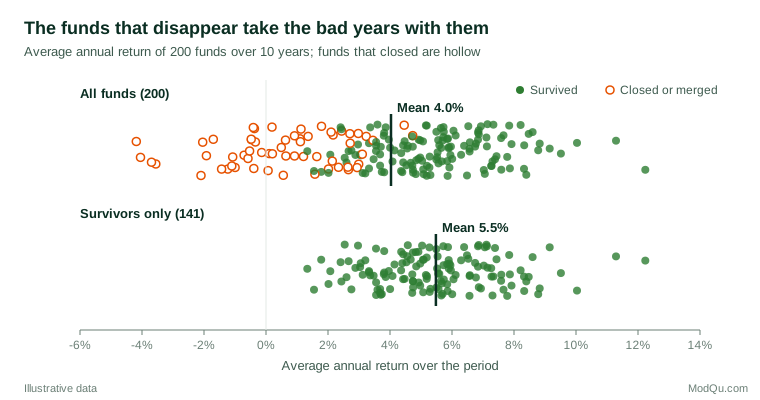
Investment performance is the best documented business example. Funds that perform badly are often closed or merged into other funds, and databases that list only current funds then show a history made up largely of winners. Figure 1 shows a hypothetical example. Of 200 funds launched together, 59 close within ten years, mostly those with low returns. The average annual return of all 200 funds is 4.0%; the average of the 141 survivors is 5.5%.
The effect is not limited to averages. Brown et al. (1992) showed that survivorship can create the appearance that good performance persists from one period to the next, even when there is no true persistence, because funds with poor results are removed from the sample. Elton et al. (1996) found that funds which disappeared had performed markedly worse than those that survived, so that studies using only surviving funds overstate average performance. Analysts now use databases that keep records of closed funds for precisely this reason. Similar distortions affect stock market indices, which drop companies that fail or shrink, and statistics on new businesses drawn only from firms that are still trading. Estimates of the typical return on start-up investment, or of the typical growth path of a new business, need the full set of businesses that started, not the set that can still be found.
Business lessons from successful firms
Books and case studies about what successful companies have in common invite the same error. If only successful firms are studied, any practice they share may be equally common among firms that failed. Denrell (2003) showed formally how the undersampling of failure leads to mistaken management lessons. Risky strategies, in particular, produce both spectacular successes and many failures; when only the survivors are visible, risk-taking appears to cause success. The same applies to studies of successful product launches, high-performing sales staff or "best practice" benchmarking. Before drawing a lesson from winners, ask how many firms, products or people followed the same practice and failed.
Customers and cohorts
Survivorship bias also distorts trends over time. Customers differ in loyalty, and the least loyal leave first. A cohort's observed retention rate therefore rises month by month even if no customer's behaviour changes. Figure 2 shows a hypothetical cohort in which half the customers have a 70% chance of staying each month and half a 95% chance. Observed retention rises from 82.5% in the first month to over 94% by month 12, simply because the active base becomes dominated by the loyal group.
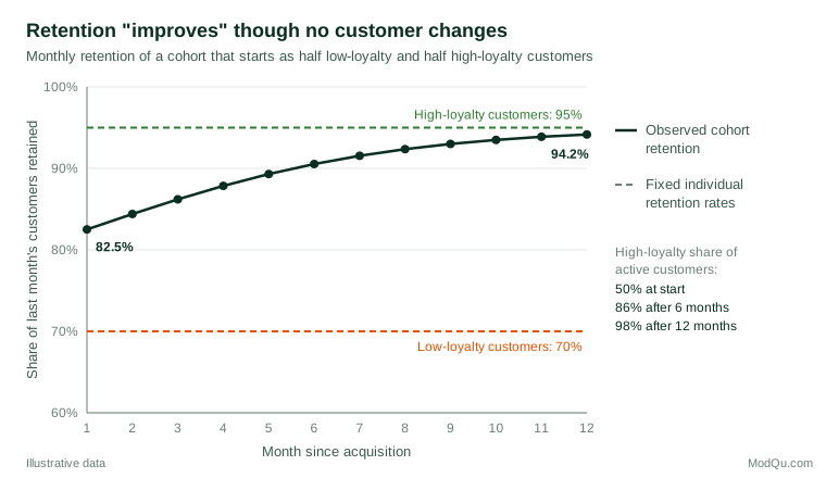
Fader and Hardie (2007) showed that this kind of heterogeneity explains why retention rates usually increase with customer tenure, and that ignoring it leads to poor projections of future retention. Demographers recognised the same effect much earlier: Vaupel et al. (1979) showed that population mortality rates can follow a very different pattern from the risks faced by individuals, because frailer individuals die first. The practical consequence is that a rising retention rate, or a rising satisfaction score among long-standing customers, is not evidence that a loyalty programme is working. Comparisons should be made between cohorts at the same tenure, or with models that allow for differences between customers.
Surveys and panels
Survey data are filtered in several ways. Customer satisfaction surveys typically reach current customers, so the views of those who have already left, often the least satisfied, are absent. Longitudinal panels lose members over time, and those who drop out may differ in the very attitudes being tracked. Nonresponse works similarly: bias arises when the likelihood of responding is related to the survey variables, and the response rate alone is a poor guide to its size (Groves & Peytcheva, 2008). Statistically, these are cases where data are missing not at random, which requires explicit assumptions about the missing cases (Little & Rubin, 2019). Suppose a subscription service surveys its current customers every year. If dissatisfied customers are more likely to cancel, the share of satisfied respondents can rise from one year to the next although the service has not improved at all. Following a fixed cohort over time, or adding exit surveys of customers who have cancelled, separates genuine change from a changing mix of respondents. The first defence is design: a sampling frame that includes former customers or lapsed panel members (Lohr, 2021).
Survival in time: immortal time bias
A subtle version arises when people or customers are classified by something that happens after the start of follow-up. Redelmeier and Singh (2001) reported that actors and actresses who won an Academy Award lived about four years longer than their nominated peers. Winners, however, must survive long enough to win, and that guaranteed survival time was credited to the winning group. Sylvestre et al. (2006) reanalysed the data, counting time before a win correctly, and found a much smaller advantage that was not statistically significant. Suissa (2008) described the same "immortal time bias" in studies of medicines, where patients are classed as users only once they fill a prescription. In business data the error appears when, for example, loyalty-card holders are compared with non-holders from the date of first purchase, although customers had to stay active long enough to sign up. Survival analysis methods, starting with the Kaplan–Meier estimator (Kaplan & Meier, 1958), handle incomplete follow-up properly when time zero is defined consistently for every group.
Detecting and correcting survivorship bias
- Define the population at the start. Ask what the full set of units was when the process began: all funds launched, all customers acquired, all products introduced.
- Find the missing records. Use archives of closed accounts, lapsed customers, discontinued products and dropped panel members. A dataset that contains only current entities should be labelled as such.
- Align time zero. Classify units by their status at a common starting point, or treat later events as time-varying.
- Compare like with like. Compare cohorts at the same age or tenure rather than survivors with newcomers.
- Model the selection. When missing cases cannot be recovered, selection models (Heckman, 1979), weighting by the estimated probability of remaining in the data, or sensitivity analyses can show how much the conclusions depend on the missing units.
- Remember the file drawer. Published studies and internal "success stories" are themselves survivors; results that disappointed are less likely to be written up (Rosenthal, 1979).
Common mistakes
- Benchmarking against the market leaders and copying their practices without checking how common those practices were among failures.
- Reporting tenure-based trends as improvements when the composition of the active base is changing.
- Treating long-standing customers' satisfaction as representative of all customers.
- Reading the absence of failures as safety. A supplier list with no recent defaults may simply have dropped the suppliers that defaulted.
- Using current lists as sampling frames for questions about the past, such as the performance of firms or products over a decade.
Key takeaways
Data rarely arrive as a complete record of everything that happened. They arrive filtered, and the filter is often survival. Whenever a dataset contains only cases that lasted, succeeded or stayed, ask what the missing cases would show and whether their absence is related to the outcome. Defining the population at the start, recovering the casualties, aligning time zero and modelling the selection turn survivorship bias from a hidden distortion into a visible and manageable source of error.
References
Brown, S. J., Goetzmann, W., Ibbotson, R. G., & Ross, S. A. (1992). Survivorship bias in performance studies. The Review of Financial Studies, 5(4), 553–580. https://doi.org/10.1093/rfs/5.4.553
Denrell, J. (2003). Vicarious learning, undersampling of failure, and the myths of management. Organization Science, 14(3), 227–243. https://doi.org/10.1287/orsc.14.3.227.15164
Elton, E. J., Gruber, M. J., & Blake, C. R. (1996). Survivor bias and mutual fund performance. The Review of Financial Studies, 9(4), 1097–1120. https://doi.org/10.1093/rfs/9.4.1097
Elwert, F., & Winship, C. (2014). Endogenous selection bias: The problem of conditioning on a collider variable. Annual Review of Sociology, 40, 31–53. https://doi.org/10.1146/annurev-soc-071913-043455
Fader, P. S., & Hardie, B. G. S. (2007). How to project customer retention. Journal of Interactive Marketing, 21(1), 76–90. https://doi.org/10.1002/dir.20074
Groves, R. M., & Peytcheva, E. (2008). The impact of nonresponse rates on nonresponse bias: A meta-analysis. Public Opinion Quarterly, 72(2), 167–189. https://doi.org/10.1093/poq/nfn011
Heckman, J. J. (1979). Sample selection bias as a specification error. Econometrica, 47(1), 153–161. https://doi.org/10.2307/1912352
Hernán, M. A., Hernández-Díaz, S., & Robins, J. M. (2004). A structural approach to selection bias. Epidemiology, 15(5), 615–625. https://doi.org/10.1097/01.ede.0000135174.63482.43
Kaplan, E. L., & Meier, P. (1958). Nonparametric estimation from incomplete observations. Journal of the American Statistical Association, 53(282), 457–481. https://doi.org/10.1080/01621459.1958.10501452
Little, R. J. A., & Rubin, D. B. (2019). Statistical analysis with missing data (3rd ed.). Wiley. https://doi.org/10.1002/9781119482260
Lohr, S. L. (2021). Sampling: Design and analysis (3rd ed.). Chapman and Hall/CRC. https://doi.org/10.1201/9780429298899
Mangel, M., & Samaniego, F. J. (1984). Abraham Wald's work on aircraft survivability. Journal of the American Statistical Association, 79(386), 259–267. https://doi.org/10.1080/01621459.1984.10478038
Redelmeier, D. A., & Singh, S. M. (2001). Survival in Academy Award–winning actors and actresses. Annals of Internal Medicine, 134(10), 955–962. https://doi.org/10.7326/0003-4819-134-10-200105150-00009
Rosenthal, R. (1979). The file drawer problem and tolerance for null results. Psychological Bulletin, 86(3), 638–641. https://doi.org/10.1037/0033-2909.86.3.638
Suissa, S. (2008). Immortal time bias in pharmacoepidemiology. American Journal of Epidemiology, 167(4), 492–499. https://doi.org/10.1093/aje/kwm324
Sylvestre, M.-P., Huszti, E., & Hanley, J. A. (2006). Do Oscar winners live longer than less successful peers? A reanalysis of the evidence. Annals of Internal Medicine, 145(5), 361–363. https://doi.org/10.7326/0003-4819-145-5-200609050-00009
Vaupel, J. W., Manton, K. G., & Stallard, E. (1979). The impact of heterogeneity in individual frailty on the dynamics of mortality. Demography, 16(3), 439–454. https://doi.org/10.2307/2061224