
Statistics · Communication and misuse
Misleading Graphs: Truncated Axes, Cherry-Picked Ranges and Dual Axes
Three of the most common ways charts mislead, each shown beside an honest version of the same data, with evidence on how readers are fooled and simple rules for drawing fair graphs.
Readers take in the shape of a chart in a fraction of a second, long before they read its axis labels. That is what makes charts so useful, and also what makes them easy to abuse. Huff (1954) called the classic example the "gee-whiz graph": a chart whose axis has been cut so that a small rise looks like a surge. Wainer (1984) later catalogued a dozen ways of "displaying data badly", and Tufte (2001) proposed a simple test of honesty, the lie factor: the size of an effect as shown in the graphic divided by its size in the data. A fair chart has a lie factor close to 1.
This article looks at three distortions that appear constantly in business reports, dashboards and the media: truncated axes, cherry-picked ranges and dual axes. Each is shown beside an honest version of the same illustrative data.
Truncated axes
In a bar chart, readers judge values by the length of the bars. Cleveland and McGill (1984) showed experimentally that people judge position and length along a common scale more accurately than angles, areas or colours, which is why bar charts work well. The corollary is that a bar's length must be proportional to its value. If the axis starts above zero, it is not.
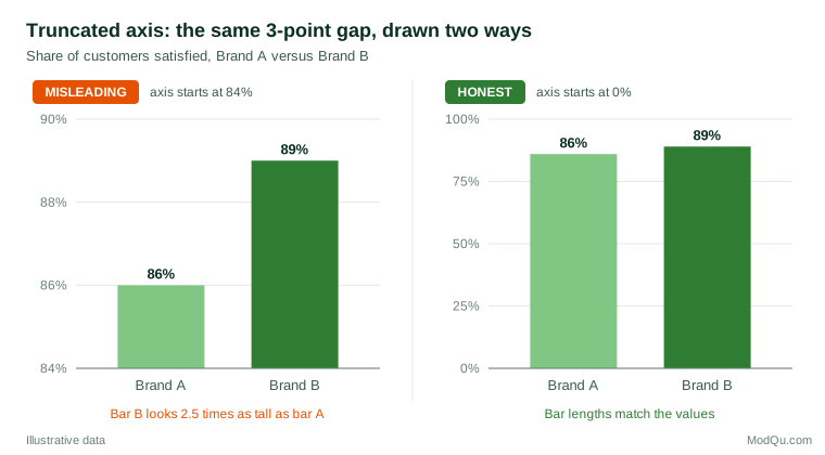
In Figure 1, Brand B's satisfaction score is 89% against Brand A's 86%, a relative difference of about 3.5%. With the axis starting at 84%, Brand B's bar is 2.5 times as long as Brand A's, an apparent difference of 150%. The lie factor is roughly 150 ÷ 3.5 ≈ 43. Readers are not protected by the printed numbers. Pandey et al. (2015) found that truncated axes led participants to judge differences as larger even when values were labelled. Correll et al. (2020) found the exaggeration for both bar and line charts, and Yang et al. (2021) showed that it persisted even after participants were told explicitly that the axis was truncated.
The rule is therefore firm for bar charts: start the axis at zero. For line charts and dot plots it is more flexible. Their message lies in position and slope rather than length, and a zero baseline can flatten meaningful variation into a straight line. Cleveland (1994) and Few (2012) both argue that a non-zero scale is acceptable for such charts, provided it is clearly labelled and chosen to show the data rather than to dramatise them. If a small difference matters, a better solution than truncating bars is to plot the difference itself, or to use dot plots that show the values and their uncertainty (Weissgerber et al., 2015).
Cherry-picked ranges
A time series can tell almost any story if the start and end dates are chosen to suit the storyteller. Seasonal businesses are particularly exposed: the peak-to-trough months of any year can be presented as a collapse, and trough-to-peak months as a boom.
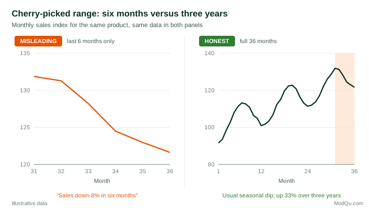
The left panel of Figure 2 shows a fall of about 8% over the last six months, drawn on a narrow scale that makes it look precipitous. The right panel shows the full 36 months. The recent fall is the same seasonal dip that occurs every year; sales in the final month were about 9% higher than a year earlier and about 33% higher than three years earlier.
Cherry-picking also works in the other direction, by starting a series at an unusually low point to manufacture growth, or by choosing the period that makes a campaign or policy look best. Cairo (2019) gives many examples from public debate, and notes that the honest question is always what a reasonable reader would conclude from a longer or different window.
Practical defences are straightforward. Show enough history to reveal trend and seasonality, typically at least two or three full cycles. Compare like with like, such as year-on-year changes for seasonal data. State why a particular start date was chosen. If only recent data matter, say so and show the longer series in an appendix.
Survey trackers deserve special care. Brand and satisfaction trackers often have small changes between waves, some of which are within the margin of error. Showing only the last two or three waves, on a narrow scale, invites readers to see movement where there is mostly sampling noise. A longer series with intervals around each wave gives a much fairer picture.
Dual axes
Dual-axis charts plot two series with different units against separate left and right scales. They are common in marketing and finance, where spend is plotted against revenue or one price against another. The problem is that the analyst can choose both scales freely, and by stretching or compressing either one can make the lines cross, diverge or overlap at will. The visual relationship between the lines then reflects the choice of scales, not the data.
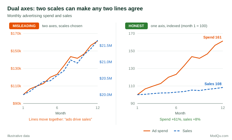
In the left panel of Figure 3, the two lines move together so closely that the chart seems to prove that advertising drives sales. In fact spend rose 61% over the year while sales rose 8%. The overlap was produced by choosing a sales axis that covers only a narrow band of values. Vigen (2015) used exactly this device to make absurd pairs of series, such as unrelated national statistics, appear to track each other, which shows how little a dual-axis overlap proves. Even when two series are related, a dual axis says nothing about causation.
Healy (2018) recommends alternatives that remove the arbitrary choice: index both series to a common starting value, as in the right panel; plot them in separate panels stacked vertically with a shared time axis; or, if the relationship itself is the point, draw a scatter plot of one against the other. If a dual axis must be used, the scales should be chosen by a stated rule, such as both starting at zero, and the axes should be coloured to match their lines.
Other distortions to watch for
The three distortions above are the most common, but not the only ones. Wainer (1984) and Tufte (2001) describe several more:
- Area and volume for one-dimensional data. Scaling an icon in height and width makes a doubling look like a fourfold increase.
- Inconsistent intervals. Uneven gaps between dates or categories distort trends.
- Hidden uncertainty. Point estimates without intervals imply more precision than the data support. Spiegelhalter et al. (2011) review clearer ways to show uncertainty.
- Three-dimensional effects. Perspective makes bars and pie slices hard to compare.
- Inverted or reversed axes. An axis that runs downward can make a rise look like a fall, an effect Pandey et al. (2015) also observed in their experiments.
A checklist for honest charts
- Bar charts start at zero; any other baseline is clearly marked and justified.
- The time window shows enough history to reveal trend and seasonality, and its choice is explained.
- Two series with different units are indexed, shown in separate panels or plotted against each other rather than on two free axes.
- Lengths and areas are proportional to the values they show.
- Uncertainty, sample sizes and data sources are shown or stated.
- The chart title states what the data show, and the chart supports that statement without exaggeration.
Key takeaways
Truncated axes, cherry-picked ranges and dual axes are popular because they make data look more dramatic, and experiments show that readers are misled even when the correct numbers are printed. Honest alternatives are easy: zero-based bars, longer windows with like-for-like comparisons, and indexed or separate panels for series in different units. A useful habit is to draw the honest version beside the dramatic one, as in this article, and ask whether the message survives. If it does not, the message was in the design rather than in the data.
References
Cairo, A. (2019). How charts lie: Getting smarter about visual information. W. W. Norton.
Cleveland, W. S. (1994). The elements of graphing data (Rev. ed.). Hobart Press.
Cleveland, W. S., & McGill, R. (1984). Graphical perception: Theory, experimentation, and application to the development of graphical methods. Journal of the American Statistical Association, 79(387), 531–554. https://doi.org/10.1080/01621459.1984.10478080
Correll, M., Bertini, E., & Franconeri, S. (2020). Truncating the y-axis: Threat or menace? In Proceedings of the 2020 CHI Conference on Human Factors in Computing Systems (pp. 1–12). ACM. https://doi.org/10.1145/3313831.3376222
Few, S. (2012). Show me the numbers: Designing tables and graphs to enlighten (2nd ed.). Analytics Press.
Healy, K. (2018). Data visualization: A practical introduction. Princeton University Press.
Huff, D. (1954). How to lie with statistics. W. W. Norton.
Pandey, A. V., Rall, K., Satterthwaite, M. L., Nov, O., & Bertini, E. (2015). How deceptive are deceptive visualizations? An empirical analysis of common distortion techniques. In Proceedings of the 33rd Annual ACM Conference on Human Factors in Computing Systems (pp. 1469–1478). ACM. https://doi.org/10.1145/2702123.2702608
Spiegelhalter, D., Pearson, M., & Short, I. (2011). Visualizing uncertainty about the future. Science, 333(6048), 1393–1400. https://doi.org/10.1126/science.1191181
Tufte, E. R. (2001). The visual display of quantitative information (2nd ed.). Graphics Press.
Vigen, T. (2015). Spurious correlations. Hachette Books.
Wainer, H. (1984). How to display data badly. The American Statistician, 38(2), 137–147. https://doi.org/10.1080/00031305.1984.10483186
Weissgerber, T. L., Milic, N. M., Winham, S. J., & Garovic, V. D. (2015). Beyond bar and line graphs: Time for a new data presentation paradigm. PLOS Biology, 13(4), Article e1002128. https://doi.org/10.1371/journal.pbio.1002128
Yang, B. W., Vargas Restrepo, C., Stanley, M. L., & Marsh, E. J. (2021). Truncating bar graphs persistently misleads viewers. Journal of Applied Research in Memory and Cognition, 10(2), 298–311. https://doi.org/10.1016/j.jarmac.2020.10.002