
Statistics · Communication and misuse
Principles of Data Visualisation for Statistical Results
How to choose and design charts that show statistical results accurately, drawing on research into graphical perception, colour and the display of uncertainty, with practical guidance for survey reports.
A good chart lets the reader see a pattern, a difference or a trend faster and more reliably than a table of numbers can. A poor one hides the pattern, or suggests one that is not there. Statistical graphics are part of the analysis, not decoration, and often the main way its findings reach decision-makers. Gelman et al. (2002) went so far as to argue that many of the tables published in statistics journals would communicate better as graphs. This article sets out the principles that research and long practice support: how charts encode numbers, which encodings people read most accurately, how to match the chart to the question, and how to show uncertainty. A companion article covers the ways graphs mislead; the emphasis here is on good practice.
Why plot the data at all?
Summary statistics can conceal very different patterns. Anscombe (1973) constructed four small data sets with the same means, variances, correlations and regression lines, yet their scatterplots looked completely different: one roughly linear, one curved, one with a single outlier, and one whose slope depended on a single extreme point. Tukey (1977) built exploratory data analysis on the same insight, urging analysts to look at data before and after modelling. For survey and business data this means plotting distributions, not only averages, and checking subgroups and time trends before reducing them to a single number.
Encoding: how charts carry numbers
Every chart maps data values to visual properties: position along an axis, the length of a bar, the angle of a pie slice, the area of a bubble or the shade of a colour. These mappings are called encodings, and they are not equally easy to read. Cleveland and McGill (1984) ran experiments in which people judged the relative sizes of values shown with different encodings, and proposed a ranking from most to least accurate:
- Position along a common scale (dot plots, bar charts with a shared baseline).
- Position along identical but non-aligned scales (the same axis repeated in separate panels).
- Length, direction and angle.
- Area.
- Volume and curvature.
- Shading and colour saturation.
Heer and Bostock (2010) repeated several of these experiments with a large online sample and obtained a broadly similar ordering, which suggests that the ranking is robust. Franconeri et al. (2021), reviewing the wider research literature on visual communication, reach the same practical conclusion: when precise comparison matters, use position or length on an aligned scale.
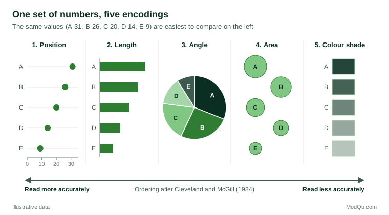
The ranking explains several familiar recommendations. A pie chart asks readers to compare angles and areas, so small differences between slices are hard to see; a sorted bar chart of the same shares makes them plain. Bubble charts and shaded maps give a useful overview but poor exact comparison, so key values should also be labelled or tabulated. Three-dimensional effects add volume and perspective, the least accurate cues, and no information.
Matching the chart to the question
The best chart depends on the comparison the reader needs to make. A useful habit is to write that comparison down in one sentence before choosing the form.
| Question | Usually effective form |
|---|---|
| How do categories compare? | Sorted horizontal bar chart or dot plot |
| How has a measure changed over time? | Line chart |
| How are values distributed? | Histogram, box plot or plot of individual values |
| How do two continuous variables relate? | Scatterplot, with a smoothed trend if helpful |
| How do parts make up a whole? | Stacked bar, or bar chart of shares |
| How do patterns differ across many groups? | Small multiples on a common scale |
Bar charts should start at zero, because the reader judges the length of each bar; dot plots and line charts need not, because the reader judges position. Horizontal bars leave room for long category labels such as survey answer options. Tufte (2001) recommended small multiples, a grid of small charts with identical axes, so that the eye can compare panels directly; this usually works better than one crowded chart with many coloured lines.
For continuous outcomes, bar charts of means are a weak choice. Weissgerber et al. (2015) showed that very different data sets, including ones with outliers, skew or two distinct clusters, can produce identical bar graphs, and recommended plots that show individual observations or the full distribution, especially for small samples. The box plot, introduced by Tukey (1977) and extended by McGill et al. (1978) with variable widths and notches, summarises the median, quartiles and unusual values compactly. Krzywinski and Altman (2014) advise stating the sample size and how the whiskers are defined, because conventions differ between software packages.
Design details that matter
Tufte (2001) urged designers to devote as much of the ink as possible to the data and to remove "chartjunk": heavy gridlines, background images, unnecessary borders and decorative effects. Extreme minimalism can strip away useful context, but the core advice holds: every element should help the reader.
- Label directly. Place series names at the ends of lines rather than in a separate legend where possible.
- Order meaningfully. Sort categories by value unless they have a natural order, such as age bands or a Likert scale, which should keep that order.
- Use colour with purpose. Harrower and Brewer (2003) distinguish sequential schemes for ordered values, diverging schemes for values either side of a meaningful midpoint, and qualitative schemes for unordered categories. A diverging scheme suits agree–disagree scales; a qualitative scheme suits brands. Use one highlight colour for the key result and grey for context, and choose colours that stay distinguishable for readers with colour-vision deficiency.
- Write informative titles. A title that states the finding ("Satisfaction rose in every region") tells readers what to look for; axis labels and the caption should give the measure, units, base and source.
- Keep scales consistent. Charts that will be compared should share their axes.
Wainer (1984) described the opposite habits, such as showing as few data as possible and ordering categories alphabetically, in an ironic guide to displaying data badly that remains a useful checklist of what to avoid.
Showing uncertainty
Survey estimates and model results carry sampling error, and a chart that shows only point estimates invites readers to over-interpret small differences. The usual remedy is to plot each estimate with an interval, typically a 95% confidence interval.
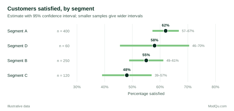
Intervals help, but they are easily misread. Belia et al. (2005) found that many published researchers misjudged how far apart error bars must be for a difference to be statistically significant, and often failed to distinguish standard-error bars from confidence intervals. Cumming and Finch (2005) offer rules of thumb for two independent groups: when two 95% confidence intervals overlap by no more than about half the average margin of error, the difference is roughly significant at the 5% level, and when they just touch it is significant at about the 1% level. It follows that overlapping intervals do not, on their own, show that there is no difference. Every chart with error bars should state what the bars represent.
Other displays convey uncertainty more intuitively. Fan charts, used by central banks for inflation projections, show bands of decreasing probability around a central path, and Spiegelhalter et al. (2011) review these alongside icon arrays and other formats for presenting risk and uncertainty. Hullman et al. (2015) found that hypothetical outcome plots, animations that show a sequence of plausible draws, helped people judge how likely one value was to exceed another more accurately than error bars or violin plots did. For printed reports, shaded bands and plain statements such as "the true figure is likely to lie between 49% and 61%" are practical options.
Practical guidance for survey reports
- Plot weighted estimates, and base intervals on design-aware standard errors rather than the raw sample size.
- Show the unweighted base for each group, and flag or suppress estimates from very small bases.
- Use dot plots with intervals for comparing segments, and diverging stacked bars for full Likert distributions.
- When tracking a metric over time, show intervals or a band so that readers do not react to month-to-month noise.
- Pair each chart with a sentence that states the main finding and its uncertainty.
Common mistakes
- Choosing the chart type from software defaults rather than from the question.
- Using pie charts with many slices or with similar shares.
- Showing bar charts of means that hide skewed or clustered data.
- Leaving error bars unexplained, or reading any overlap as "no difference".
- Using colour scales that imply an order where there is none, or a rainbow scale for ordered data.
Key takeaways
Effective statistical graphics start from the question the reader needs to answer. Encode the most important comparison as position on a common scale, show distributions rather than only averages, remove clutter, use colour deliberately and display uncertainty with clearly labelled intervals or bands. Charts designed this way let business audiences see what the data show and how confident they can be about it.
References
Anscombe, F. J. (1973). Graphs in statistical analysis. The American Statistician, 27(1), 17–21. https://doi.org/10.1080/00031305.1973.10478966
Belia, S., Fidler, F., Williams, J., & Cumming, G. (2005). Researchers misunderstand confidence intervals and standard error bars. Psychological Methods, 10(4), 389–396. https://doi.org/10.1037/1082-989X.10.4.389
Cleveland, W. S., & McGill, R. (1984). Graphical perception: Theory, experimentation, and application to the development of graphical methods. Journal of the American Statistical Association, 79(387), 531–554. https://doi.org/10.1080/01621459.1984.10478080
Cumming, G., & Finch, S. (2005). Inference by eye: Confidence intervals and how to read pictures of data. American Psychologist, 60(2), 170–180. https://doi.org/10.1037/0003-066X.60.2.170
Franconeri, S. L., Padilla, L. M., Shah, P., Zacks, J. M., & Hullman, J. (2021). The science of visual data communication: What works. Psychological Science in the Public Interest, 22(3), 110–161. https://doi.org/10.1177/15291006211051956
Gelman, A., Pasarica, C., & Dodhia, R. (2002). Let's practice what we preach: Turning tables into graphs. The American Statistician, 56(2), 121–130. https://doi.org/10.1198/000313002317572790
Harrower, M., & Brewer, C. A. (2003). ColorBrewer.org: An online tool for selecting colour schemes for maps. The Cartographic Journal, 40(1), 27–37. https://doi.org/10.1179/000870403235002042
Heer, J., & Bostock, M. (2010). Crowdsourcing graphical perception: Using Mechanical Turk to assess visualization design. In Proceedings of the SIGCHI Conference on Human Factors in Computing Systems (pp. 203–212). Association for Computing Machinery. https://doi.org/10.1145/1753326.1753357
Hullman, J., Resnick, P., & Adar, E. (2015). Hypothetical outcome plots outperform error bars and violin plots for inferences about reliability of variable ordering. PLOS ONE, 10(11), Article e0142444. https://doi.org/10.1371/journal.pone.0142444
Krzywinski, M., & Altman, N. (2014). Visualizing samples with box plots. Nature Methods, 11(2), 119–120. https://doi.org/10.1038/nmeth.2813
McGill, R., Tukey, J. W., & Larsen, W. A. (1978). Variations of box plots. The American Statistician, 32(1), 12–16. https://doi.org/10.1080/00031305.1978.10479236
Spiegelhalter, D., Pearson, M., & Short, I. (2011). Visualizing uncertainty about the future. Science, 333(6048), 1393–1400. https://doi.org/10.1126/science.1191181
Tufte, E. R. (2001). The visual display of quantitative information (2nd ed.). Graphics Press.
Tukey, J. W. (1977). Exploratory data analysis. Addison-Wesley.
Wainer, H. (1984). How to display data badly. The American Statistician, 38(2), 137–147. https://doi.org/10.1080/00031305.1984.10483186
Weissgerber, T. L., Milic, N. M., Winham, S. J., & Garovic, V. D. (2015). Beyond bar and line graphs: Time for a new data presentation paradigm. PLOS Biology, 13(4), Article e1002128. https://doi.org/10.1371/journal.pbio.1002128