
Statistics · Foundations
Populations, Samples, Parameters and Statistics
The four ideas behind every survey estimate: what a population and a sample are, how a parameter differs from a statistic, and why sample quality matters more than sample size.
Every survey result answers a question about a group of people who were not all asked. When a report says that 63% of customers would recommend a brand, it uses the answers of a few hundred people to describe thousands or millions. Four terms make that leap possible and keep it honest: population, sample, parameter and statistic. They sound elementary, yet confusion between them lies behind many costly errors in business research: polls that ask the wrong people, dashboards that treat a sample figure as a fact, and very large data sets that prove less informative than small random ones. This article defines each idea, works through an example and sets out practical guidance.
Four ideas in one sentence
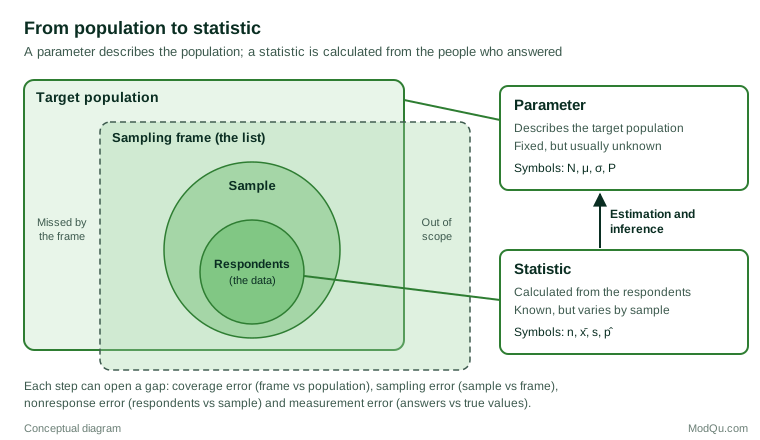
A population is the complete set of units we want to learn about. A sample is the subset of those units we actually observe. A parameter is a number that describes the population, such as the true percentage of all customers who would recommend us. A statistic is a number calculated from the sample, such as the percentage of surveyed customers who said they would. In one sentence: we calculate statistics from samples in order to estimate parameters of populations.
The vocabulary goes back to R. A. Fisher, who in a founding paper of modern statistics separated the quantities that characterise a population, which he called parameters, from the quantities calculated from data to estimate them, which he called statistics (Fisher, 1922). The distinction matters because the two kinds of number behave very differently. A parameter is fixed at any moment, but we usually do not know it. A statistic is known as soon as the data are in, but it would have come out differently had a different sample been drawn.
The population: deciding what you want to know
Defining the population is a business decision before it is a statistical one. "Our customers" might mean everyone who bought in the past year, everyone with an active account, or every household that could buy. Each choice defines a different parameter. Survey textbooks therefore distinguish several related populations (Lohr, 2021; Statistics Canada, 2010):
- The target population is the group the decision is about, defined by who is included, where and when, for example "adults in Canada who bought a mobile phone plan in the past 12 months".
- The survey population or sampled population is the part of the target population that the survey can actually reach.
- The sampling frame is the list or procedure used to select units, such as a customer database, a list of addresses or a panel. Frames are rarely perfect. Some members of the target population are missing from them (undercoverage), and some entries do not belong (overcoverage, duplicates or out-of-scope units).
It also helps to be clear about the unit. A survey may select households but measure individuals, or select stores but measure transactions. A parameter about "the average customer" is different from one about "the average purchase", because heavy buyers count once in the first and many times in the second.
Finite populations and processes
Many business populations are finite and can, in principle, be listed: the 20,000 members of a loyalty programme, or every invoice issued last quarter. Other questions concern a process rather than a list. A manager who asks whether a new checkout design will raise conversion is asking about future visitors who do not yet exist. Deming (1953) called the first kind of study enumerative, because it aims to describe a defined, existing population, and the second analytic, because it aims to understand the causes that will shape future results. Hahn and Meeker (1993) stress that standard statistical intervals quantify only the uncertainty of an enumerative kind. When the real population of interest is a future one, the analyst must also assume that the process will remain stable, and no formula can check that assumption.
Parameters: fixed but unknown
A parameter is a summary of the whole population. Common examples are the population mean (written μ), the population standard deviation (σ), a population proportion (written P, or sometimes π), a population total, and a regression slope that would be obtained if every member of the population were measured. In market research the parameters of interest are often proportions and totals: the share of the market aware of a brand, the number of households intending to switch supplier, or the mean amount spent per visit.
Two features of parameters are easy to forget. First, a parameter is defined by the population, the variable and the time. "Satisfaction among active subscribers in March, on a ten-point scale" is a parameter; "customer satisfaction" is not. Second, a parameter belongs to the population, not to the survey. A better survey does not change it; it only brings the estimate closer.
Samples and statistics
A statistic is any quantity calculated from sample data. The sample mean (x̄), the sample standard deviation (s), the sample proportion (p̂, read "p-hat") and a fitted regression coefficient are all statistics. So, less obviously, are test statistics and p-values. A statistic used to estimate a parameter is called an estimator when we think of it as a rule, and an estimate when we mean the particular number a survey produced.
The conventional notation helps to keep the two worlds apart: Greek letters or capitals for the population, Latin letters for the sample.
| Quantity | Population (parameter) | Sample (statistic) |
|---|---|---|
| Size | N | n |
| Mean | μ | x̄ |
| Standard deviation | σ | s |
| Proportion | P (or π) | p̂ |
| Regression slope | β | b (or β̂) |
A census measures every unit, so in principle its figures are parameters. In practice, censuses and customer databases still contain missing records and coding errors, so even "complete" data deserve scrutiny.
Sampling variability and the sampling distribution
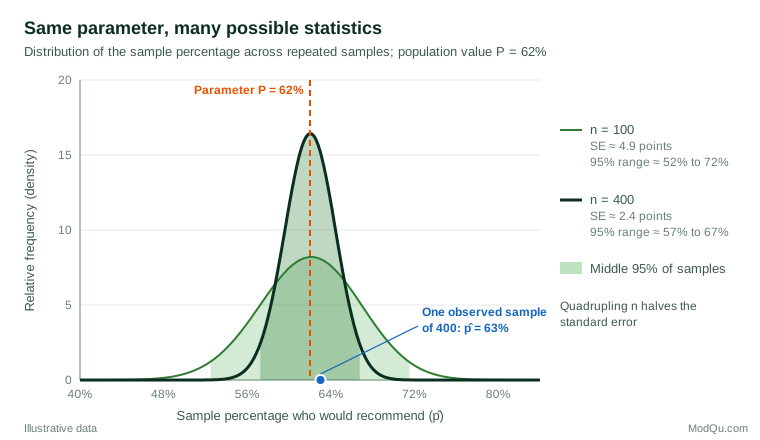
If we drew a second sample from the same population, we would almost certainly get a slightly different statistic. The pattern of values a statistic would take over all the samples a design could produce is called its sampling distribution. It is the bridge between a single result and the unknown parameter. Student (1908) worked out the sampling distribution of the mean for small samples, the basis of the t test, and Efron (1979) later showed how to approximate sampling distributions by resampling the observed data when no formula is available.
The spread of the sampling distribution is measured by the standard error. For a proportion estimated from a simple random sample, it is:
SE(p̂) = √[P(1 − P) ÷ n] × √(1 − n ÷ N)
The second term, the finite population correction, matters only when the sample is a sizeable fraction of the population. With 400 people drawn from 20,000, it equals about 0.99 and can usually be ignored. The first term carries the main lesson: precision depends on the absolute size of the sample, not on the share of the population sampled, and it improves only with the square root of n. Quadrupling the sample halves the standard error.
A worked example
Consider a hypothetical retailer with a loyalty programme of N = 20,000 members. Management wants to know what proportion of members would recommend the retailer to a friend. That proportion, P, is the parameter. Suppose, for the purpose of illustration, that the true value is 62%. Nobody in the company knows this.
The research team draws a simple random sample of n = 400 members from the programme list, which serves as the sampling frame, and all 400 answer. Of these, 252 say they would recommend the retailer, so the statistic is p̂ = 252 ÷ 400 = 63%. The estimated standard error, using p̂ in place of the unknown P and including the finite population correction, is:
SE = √[0.63 × 0.37 ÷ 400] × √(1 − 400 ÷ 20,000) ≈ 0.024
A 95% confidence interval is therefore 63% ± 1.96 × 2.4 points, or about 58.3% to 67.7%. In this illustration the interval contains the true 62%, as about 95% of intervals built this way will. Figure 2 shows where this sample sits among all the samples that could have been drawn. With a sample of 100, the interval would have been about twice as wide; with 1,600 it would have been about half as wide.
Three points stand out. First, the 63% is a statistic; the 62% is the parameter. The one-point gap is sampling error, whose size the company will never know, only its likely range. Second, the interval describes the uncertainty from sampling alone. If the programme list missed members who joined online, or if dissatisfied members were less willing to answer, the interval would not reveal it. Third, the interval is a statement about the population of 20,000 members at the time of the survey. Using it to predict what next year's members will say is an analytic step that needs further assumptions (Deming, 1953).
Why sample quality beats sample size
The formulas above assume a probability sample, in which every unit on the frame has a known, non-zero chance of selection. Neyman (1934) set out the case for random and stratified selection over purposive choice of "typical" units, and introduced the confidence interval as the way to express the resulting uncertainty. Horvitz and Thompson (1952) later showed how to estimate population totals without bias when units have unequal but known selection probabilities, by weighting each response by the inverse of its probability. This design-based approach is the foundation of official statistics and most professional survey practice (Särndal et al., 1992).
When selection is not random, size offers little protection. The best-known example is the Literary Digest poll of 1936, which mailed millions of ballots and confidently predicted that Alf Landon would defeat Franklin Roosevelt. Roosevelt won by a landslide. Using a later survey that asked people whether they had taken part in the poll, Squire (1988) found that both the magazine's initial sample and the pattern of who returned their ballots favoured Landon, and that the combination produced the error.
Meng (2018) gave the problem a precise form. The error of an estimate from a non-random sample depends on the correlation between whether a unit is included and the value being measured, on the fraction of the population included, and on the variability in the population. Even a very small correlation can overwhelm a huge sample. In his analysis of the 2016 United States presidential election, a self-reported sample of about 2.3 million people, roughly 1% of eligible voters, with a selection correlation of only about −0.005, had the same mean squared error as a simple random sample of about 400. The practical message for anyone working with web analytics, transaction logs or opt-in panels is that "big" should be judged by how the data were selected, not by the row count.
Probability and non-probability samples
Probability samples are increasingly expensive, and response rates have fallen across many survey modes (Brick, 2011). Much market research therefore uses non-probability samples, such as opt-in online panels, river sampling or customer feedback forms. These can be valuable, but the link from statistic to parameter then rests on modelling assumptions rather than on the selection design.
The American Association for Public Opinion Research task force on non-probability sampling concluded that there is no single framework that justifies inference from all such samples, and that their validity depends on how well the assumptions behind the adjustments hold (Baker et al., 2013). Bethlehem (2010) showed how undercoverage of people without internet access and self-selection of volunteers can bias web survey estimates, and how weighting may reduce but not always remove that bias. Elliott and Valliant (2017) review the two main routes to inference: estimating pseudo-selection probabilities so that the sample can be weighted as if it were random, and modelling the outcome directly so that predictions can be made for the unsampled part of the population.
Model-based approaches can work well. Wang et al. (2015) used an opt-in poll of video game platform users, heavily skewed towards young men, and after multilevel regression and poststratification produced election forecasts comparable with leading poll averages. Success depended on rich demographic data and careful modelling. The debate between design-based and model-based inference is long-standing: Hansen et al. (1983) showed that model-dependent estimates can be seriously biased when the model is even slightly wrong, while Little (2004) argued for models that are calibrated to the sample design. For a business reader the lesson is simple. With a probability sample, the design does much of the work of linking statistic to parameter. Without one, the analyst's assumptions do that work, and they should be stated.
Error beyond sampling
The gap between a statistic and its parameter has more sources than chance selection. The total survey error framework groups them into errors of representation (coverage, sampling and nonresponse) and errors of measurement (questions that are misunderstood, answers that are misreported, and data processing mistakes) (Groves & Lyberg, 2010). Figure 1 marks where each enters.
Two findings are especially relevant to commercial surveys. First, a low response rate is not by itself proof of bias, nor a high one proof of accuracy. A review of studies in which bias could be measured found that the response rate was a poor predictor of nonresponse bias; what matters is whether the reasons for not responding are related to the variable being measured (Groves, 2006). Second, measurement error does not shrink as the sample grows. In a study that compared survey answers with university records, Kreuter et al. (2008) found that reporting of sensitive information, such as poor academic performance, varied by survey mode, with self-administered web questionnaires producing more accurate reports than interviewer-administered telephone interviews. A larger sample would have estimated the misreported figure more precisely, not corrected it.
When your data are the whole population
Businesses increasingly hold data on every customer or every transaction. Does that turn statistics into parameters? For an enumerative question about a defined period, largely yes: the total revenue from last quarter's invoices is a parameter, and a margin of error around it would be meaningless, although data quality still matters. But many questions that use complete data are really analytic. Comparing the purchase rates of customers who did and did not receive a promotion is usually an attempt to learn about the effect of the promotion on future customers, and then the observed customers are best seen as a sample from a wider process or "superpopulation".
This is also where p-values cause confusion. A p-value is a statistic calculated from the data under a model. It does not measure the probability that a hypothesis is true or that the data arose by chance alone, and it does not measure the size or importance of an effect (Wasserstein & Lazar, 2016). With very large data sets, trivial differences become "statistically significant". The relevant questions are whether the population and parameter have been defined clearly, and whether the difference is large enough to matter.
Practical guidance for survey and business data
- Write the parameter down before collecting data. State the target population, the variable, the time period and the summary (mean, proportion, total).
- Compare the frame with the target population. Identify who is missing (for example, customers without email addresses) and who should not be there (lapsed or duplicate accounts). Coverage gaps are rarely fixed by weighting alone.
- Prefer probability selection where possible, even a simple random draw from a customer list. Where it is not possible, record how respondents were recruited and what adjustments were made (Baker et al., 2013).
- Report the statistic with its uncertainty, and say clearly that the interval reflects sampling error only.
- Use design-aware estimation. Stratification, clustering and weights change standard errors; software for complex surveys handles them correctly (Lumley, 2010). Weighting and sample design are covered in detail by Valliant et al. (2018).
- Plan sample size around the subgroups that matter. If decisions depend on a segment that makes up 10% of the population, a total sample of 400 yields only about 40 respondents in that segment.
- Judge large data sets by how they were generated. Ask who could and could not appear in the data, and whether that is related to the outcome (Meng, 2018).
Common mistakes
- Treating a statistic as a parameter. Reporting that "63% of members would recommend us" without any reference to the sample hides the uncertainty. "An estimated 63%, with a margin of error of about five points" is more accurate.
- Defining the population after the fact. Adjusting the definition to match whoever happened to respond turns a sample of the wrong people into an apparently "complete" picture of an invented population.
- Believing a larger sample cures bias. A larger sample reduces sampling error only. Coverage, nonresponse and measurement errors remain, and their relative importance grows as the sample grows.
- Generalising beyond the population sampled. A survey of current customers says little about non-customers or about next year's market without further evidence.
Key takeaways
Populations and parameters describe what a decision needs to know; samples and statistics describe what the research actually observed. The quality of the link between them, more than the size of the sample, determines whether a survey result can be trusted. Define the target population and parameter precisely, check the frame for gaps, use probability selection where possible, and report every statistic with its uncertainty and its limitations. Judge very large data sets by how they were generated, not by how many rows they contain.
References
Baker, R., Brick, J. M., Bates, N. A., Battaglia, M., Couper, M. P., Dever, J. A., Gile, K. J., & Tourangeau, R. (2013). Summary report of the AAPOR task force on non-probability sampling. Journal of Survey Statistics and Methodology, 1(2), 90–143. https://doi.org/10.1093/jssam/smt008
Bethlehem, J. (2010). Selection bias in web surveys. International Statistical Review, 78(2), 161–188. https://doi.org/10.1111/j.1751-5823.2010.00112.x
Brick, J. M. (2011). The future of survey sampling. Public Opinion Quarterly, 75(5), 872–888. https://doi.org/10.1093/poq/nfr045
Deming, W. E. (1953). On the distinction between enumerative and analytic surveys. Journal of the American Statistical Association, 48(262), 244–255. https://doi.org/10.1080/01621459.1953.10483470
Efron, B. (1979). Bootstrap methods: Another look at the jackknife. The Annals of Statistics, 7(1), 1–26. https://doi.org/10.1214/aos/1176344552
Elliott, M. R., & Valliant, R. (2017). Inference for nonprobability samples. Statistical Science, 32(2), 249–264. https://doi.org/10.1214/16-STS598
Fisher, R. A. (1922). On the mathematical foundations of theoretical statistics. Philosophical Transactions of the Royal Society of London. Series A, Containing Papers of a Mathematical or Physical Character, 222(594–604), 309–368. https://doi.org/10.1098/rsta.1922.0009
Groves, R. M. (2006). Nonresponse rates and nonresponse bias in household surveys. Public Opinion Quarterly, 70(5), 646–675. https://doi.org/10.1093/poq/nfl033
Groves, R. M., & Lyberg, L. (2010). Total survey error: Past, present, and future. Public Opinion Quarterly, 74(5), 849–879. https://doi.org/10.1093/poq/nfq065
Hahn, G. J., & Meeker, W. Q. (1993). Assumptions for statistical inference. The American Statistician, 47(1), 1–11. https://doi.org/10.1080/00031305.1993.10475924
Hansen, M. H., Madow, W. G., & Tepping, B. J. (1983). An evaluation of model-dependent and probability-sampling inferences in sample surveys. Journal of the American Statistical Association, 78(384), 776–793. https://doi.org/10.1080/01621459.1983.10477018
Horvitz, D. G., & Thompson, D. J. (1952). A generalization of sampling without replacement from a finite universe. Journal of the American Statistical Association, 47(260), 663–685. https://doi.org/10.1080/01621459.1952.10483446
Kreuter, F., Presser, S., & Tourangeau, R. (2008). Social desirability bias in CATI, IVR, and web surveys: The effects of mode and question sensitivity. Public Opinion Quarterly, 72(5), 847–865. https://doi.org/10.1093/poq/nfn063
Little, R. J. (2004). To model or not to model? Competing modes of inference for finite population sampling. Journal of the American Statistical Association, 99(466), 546–556. https://doi.org/10.1198/016214504000000467
Lohr, S. L. (2021). Sampling: Design and analysis (3rd ed.). Chapman and Hall/CRC. https://doi.org/10.1201/9780429298899
Lumley, T. (2010). Complex surveys: A guide to analysis using R. Wiley. https://doi.org/10.1002/9780470580066
Meng, X.-L. (2018). Statistical paradises and paradoxes in big data (I): Law of large populations, big data paradox, and the 2016 US presidential election. The Annals of Applied Statistics, 12(2), 685–726. https://doi.org/10.1214/18-AOAS1161SF
Neyman, J. (1934). On the two different aspects of the representative method: The method of stratified sampling and the method of purposive selection. Journal of the Royal Statistical Society, 97(4), 558–625. https://doi.org/10.2307/2342192
Särndal, C.-E., Swensson, B., & Wretman, J. (1992). Model assisted survey sampling. Springer. https://doi.org/10.1007/978-1-4612-4378-6
Squire, P. (1988). Why the 1936 Literary Digest poll failed. Public Opinion Quarterly, 52(1), 125–133. https://doi.org/10.1086/269085
Statistics Canada. (2010). Survey methods and practices (Catalogue No. 12-587-X). https://www150.statcan.gc.ca/n1/en/catalogue/12-587-X
Student. (1908). The probable error of a mean. Biometrika, 6(1), 1–25. https://doi.org/10.1093/biomet/6.1.1
Valliant, R., Dever, J. A., & Kreuter, F. (2018). Practical tools for designing and weighting survey samples (2nd ed.). Springer. https://doi.org/10.1007/978-3-319-93632-1
Wang, W., Rothschild, D., Goel, S., & Gelman, A. (2015). Forecasting elections with non-representative polls. International Journal of Forecasting, 31(3), 980–991. https://doi.org/10.1016/j.ijforecast.2014.06.001
Wasserstein, R. L., & Lazar, N. A. (2016). The ASA statement on p-values: Context, process, and purpose. The American Statistician, 70(2), 129–133. https://doi.org/10.1080/00031305.2016.1154108