
Statistics · Tests and models
Graphical Models for Conditional Independence Knowledge Structures
How graphical models use pictures of nodes and edges to describe which variables are directly linked and which are independent once others are known, and how to use them in survey and market research.
Many questions in research are really questions about structure. Does price affect satisfaction directly, or only through perceived value? Are recommendation and repurchase linked to each other, or only because both depend on satisfaction? Which survey items belong together, and which are connected only through a third item? Graphical models answer such questions by drawing a picture. Each variable is a node, and the lines between nodes show which variables are directly related. A missing line is a statement of conditional independence: the two variables are unrelated once certain other variables are taken into account.
The idea brings together probability theory and graph theory. Dawid (1979) gave conditional independence a formal language of its own, and work by Pearl (1988) and by Lauritzen and Spiegelhalter (1988) showed how a graph can encode a whole set of such independence statements and make computation with large probability models practical. Koller and Friedman (2009) provide a comprehensive textbook treatment.
Conditional independence
Two variables A and C are conditionally independent given B if, once B is known, learning A tells nothing more about C. Ice cream sales and drownings both rise in summer; given the temperature, they are unrelated. Conditional independence is what makes complex models manageable. A joint distribution over twenty survey items has an enormous number of possible dependencies; if most pairs are independent given the others, the model needs only a fraction of them, and the remaining links are the ones worth interpreting.
Two kinds of graph
Undirected graphs, also called Markov random fields or Markov networks, connect variables with plain lines. The rule for reading them is simple: two variables are independent given all the others if no line joins them directly. For variables that follow a multivariate normal distribution, the graph corresponds exactly to the zero pattern in the inverse of the covariance matrix, also called the precision matrix. Dempster (1972) proposed estimating covariance structures by setting selected elements of this matrix to zero, an approach known as covariance selection. Each non-zero element corresponds to a partial correlation, the correlation between two variables after removing the linear influence of all the others.
Directed acyclic graphs (DAGs), often called Bayesian networks, use arrows and allow no cycles. A DAG factorises the joint distribution into a product of local pieces, each variable given its parents. Reading independence from a DAG requires a rule called d-separation (Pearl, 1988; Lauritzen et al., 1990), which rests on three basic patterns shown in Figure 1.
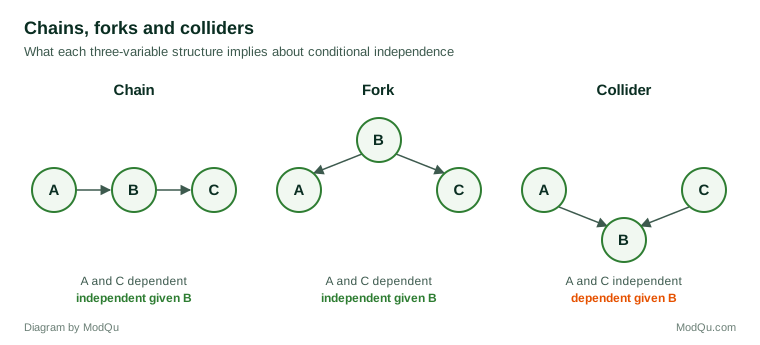
In a chain (A → B → C) and a fork (A ← B → C), A and C are associated, but the association disappears once B is held fixed. In a collider (A → B ← C), the reverse happens: A and C are unrelated, but become related once B is held fixed. Colliders explain many surprising patterns in data. If a survey only includes customers who complained (B), and complaints are caused both by product faults (A) and by poor service (C), then among complainers, faults and poor service will appear negatively related, even though they are unrelated in the full customer base. Elwert and Winship (2014) describe how conditioning on a collider, through sample selection or through adding the wrong control variable, produces this kind of bias.
Graphs as a tool for computation
Conditional independence also makes calculation possible. Once a Bayesian network has been specified, it can answer questions such as "given that this customer rated service poorly and has not repurchased, how likely is it that they will recommend us?" Without the graph, answering this would require the full joint distribution of every variable, which grows exponentially with the number of variables. With the graph, the calculation can be broken into small local steps that pass information between neighbouring nodes. Lauritzen and Spiegelhalter (1988) showed how to organise these local computations, and the method made expert systems for medical diagnosis practical. The same ideas now underlie spam filters, recommendation engines and risk models, and they explain why a well-chosen graph is valuable even when causal interpretation is not the goal (Koller & Friedman, 2009).
Learning a graph from data
When the structure is unknown, it can be estimated. For undirected graphs with continuous data, the standard tool is the graphical lasso (Friedman et al., 2008), which estimates a sparse precision matrix by penalising the size of its elements, so that weak partial correlations are set exactly to zero. Meinshausen and Bühlmann (2006) proposed a closely related approach that regresses each variable on all the others with a lasso penalty and joins two variables if either regression selects the other. Both methods work even when the number of variables is large relative to the sample size.
For directed graphs, two families of methods exist. Constraint-based methods, such as the PC algorithm, run a sequence of conditional independence tests and assemble a graph consistent with the results (Spirtes et al., 2000). Score-based methods search over possible graphs for the one that best balances fit and complexity, often with a Bayesian score that can combine prior expert knowledge with data (Heckerman et al., 1995). Glymour et al. (2019) review these and newer approaches. An important limitation is that data alone usually cannot fix the direction of every arrow: several DAGs can imply exactly the same independencies. These form an equivalence class, and only colliders and some of their consequences are identifiable from observational data.
A worked example: a customer survey network
Figure 2 shows a network estimated from simulated responses to a customer survey with seven measures: perceived price, value, product quality, service, overall satisfaction, likelihood to recommend and repurchase intention. Lines show partial correlations larger than 0.10 in absolute value.
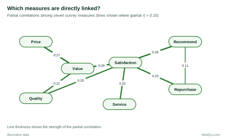
The ordinary correlation table would show every measure correlated with every other, which is common in survey data and hard to interpret. The network is sparser and tells a clearer story. Price and satisfaction have a small marginal correlation (0.10), but no direct link: price affects satisfaction only through perceived value. Service and recommendation are correlated (0.07), but the relationship runs through satisfaction. Recommendation and repurchase are directly linked only weakly (0.11), even though their ordinary correlation is larger (0.19), because much of their shared variation comes from satisfaction. For a business, the implication is that improving perceived value, quality and service matters through their effect on satisfaction, and that a campaign aimed directly at recommendation without addressing satisfaction is unlikely to change repurchase.
Network analyses of this kind are now widely used in psychology, where symptoms of a disorder are treated as a system of directly interacting parts rather than as signs of a single hidden cause (Borsboom & Cramer, 2013). Epskamp et al. (2018) set out good practice for estimating such networks, including checking how stable the estimated lines and centrality measures are when the sample is resampled.
From association to cause
Undirected networks describe association, not cause. A line between value and satisfaction does not show which affects which, or whether an unmeasured variable affects both. Directed graphs can carry causal meaning when the arrows are interpreted as direct causal effects. Causal diagrams then show which variables must be adjusted for to estimate an effect without bias, and which must not be adjusted for because they are colliders or lie on the causal path (Greenland et al., 1999; Pearl, 2009). In this role, the graph is a way of writing down assumptions so that they can be checked and debated, rather than something estimated mechanically from the data.
Practical guidance
- Decide what the graph is for. Use undirected networks to describe association structure and directed graphs to state causal assumptions.
- Check the data type. Partial correlation networks assume roughly normal continuous data; ordinal survey items may need polychoric correlations or models for binary data.
- Report stability. Use resampling to show which lines and which central nodes are reliable, as small samples produce unstable networks.
- Do not read direction from undirected lines. A line means direct association given the other variables, nothing more.
- Watch for colliders. Before adding a control variable or restricting a sample, ask whether it is a common effect of the variables of interest.
- Remember what is missing. A graph only describes the variables measured; an omitted common cause can create spurious lines.
Key takeaways
Graphical models turn a large web of correlations into a picture of which variables are directly related and which are independent once others are known. Undirected networks, estimated with methods such as the graphical lasso, reveal the direct structure among survey measures. Directed graphs encode causal assumptions and show, through chains, forks and colliders, when adjusting for a variable helps and when it creates bias. Used with attention to stability and to what has not been measured, they help researchers move from long correlation tables to clear knowledge about how measures fit together.
References
Borsboom, D., & Cramer, A. O. J. (2013). Network analysis: An integrative approach to the structure of psychopathology. Annual Review of Clinical Psychology, 9, 91–121. https://doi.org/10.1146/annurev-clinpsy-050212-185608
Dawid, A. P. (1979). Conditional independence in statistical theory. Journal of the Royal Statistical Society Series B: Statistical Methodology, 41(1), 1–15. https://doi.org/10.1111/j.2517-6161.1979.tb01052.x
Dempster, A. P. (1972). Covariance selection. Biometrics, 28(1), 157–175. https://doi.org/10.2307/2528966
Elwert, F., & Winship, C. (2014). Endogenous selection bias: The problem of conditioning on a collider variable. Annual Review of Sociology, 40, 31–53. https://doi.org/10.1146/annurev-soc-071913-043455
Epskamp, S., Borsboom, D., & Fried, E. I. (2018). Estimating psychological networks and their accuracy: A tutorial paper. Behavior Research Methods, 50(1), 195–212. https://doi.org/10.3758/s13428-017-0862-1
Friedman, J., Hastie, T., & Tibshirani, R. (2008). Sparse inverse covariance estimation with the graphical lasso. Biostatistics, 9(3), 432–441. https://doi.org/10.1093/biostatistics/kxm045
Glymour, C., Zhang, K., & Spirtes, P. (2019). Review of causal discovery methods based on graphical models. Frontiers in Genetics, 10, Article 524. https://doi.org/10.3389/fgene.2019.00524
Greenland, S., Pearl, J., & Robins, J. M. (1999). Causal diagrams for epidemiologic research. Epidemiology, 10(1), 37–48. https://doi.org/10.1097/00001648-199901000-00008
Heckerman, D., Geiger, D., & Chickering, D. M. (1995). Learning Bayesian networks: The combination of knowledge and statistical data. Machine Learning, 20(3), 197–243. https://doi.org/10.1007/BF00994016
Koller, D., & Friedman, N. (2009). Probabilistic graphical models: Principles and techniques. MIT Press.
Lauritzen, S. L., Dawid, A. P., Larsen, B. N., & Leimer, H.-G. (1990). Independence properties of directed Markov fields. Networks, 20(5), 491–505. https://doi.org/10.1002/net.3230200503
Lauritzen, S. L., & Spiegelhalter, D. J. (1988). Local computations with probabilities on graphical structures and their application to expert systems. Journal of the Royal Statistical Society Series B: Statistical Methodology, 50(2), 157–194. https://doi.org/10.1111/j.2517-6161.1988.tb01721.x
Meinshausen, N., & Bühlmann, P. (2006). High-dimensional graphs and variable selection with the lasso. The Annals of Statistics, 34(3), 1436–1462. https://doi.org/10.1214/009053606000000281
Pearl, J. (1988). Probabilistic reasoning in intelligent systems: Networks of plausible inference. Morgan Kaufmann. https://doi.org/10.1016/C2009-0-27609-4
Pearl, J. (2009). Causality: Models, reasoning, and inference (2nd ed.). Cambridge University Press. https://doi.org/10.1017/CBO9780511803161
Spirtes, P., Glymour, C., & Scheines, R. (2000). Causation, prediction, and search (2nd ed.). MIT Press. https://doi.org/10.7551/mitpress/1754.001.0001