
Statistics · Foundations
Frequentist and Bayesian Statistics: Two Philosophies of Probability
What probability means to frequentist and Bayesian statisticians, how each school turns survey data into conclusions, a worked example on purchase intention, and when each approach serves business decisions best.
Two analysts can look at the same survey and reach their conclusions in different languages. One reports that the result is "statistically significant at the 5% level" with a 95% confidence interval. The other reports that there is "a 91% probability that the true rate exceeds 15%". Both may be correct. The difference lies in what each means by probability, a question that has divided statisticians for two centuries. Understanding the two philosophies, frequentist and Bayesian, helps readers interpret reports and helps analysts answer the questions decision-makers actually ask.
Two meanings of probability
In the frequentist view, probability is a long-run frequency. Saying that a fair coin has a 50% chance of heads means that, over a very large number of tosses, about half will land heads. A fixed but unknown quantity, such as the true share of customers who would buy a new product, is not random: it simply has one value we do not know. It therefore makes no sense, in this view, to assign it a probability.
In the Bayesian view, probability measures a degree of belief, or uncertainty, given the available information. It can be attached to anything uncertain, including an unknown population share, a hypothesis or a one-off product launch. Bayesian analysis starts with a prior distribution expressing what is believed before seeing the data, and uses the data to update it into a posterior distribution (Gelman et al., 2013).
Neither definition is "the" correct one. Each is internally consistent, and each leads to a different set of tools.
A short history
The Bayesian approach is the older of the two. Thomas Bayes's essay on inferring an unknown probability from observed outcomes was published after his death (Bayes, 1763), and Laplace later developed "inverse probability" into a general method. In the early twentieth century, many statisticians grew uneasy about the subjective element in choosing a prior. Fisher (1922) laid out the mathematical foundations of estimation based on the likelihood, without priors. Neyman and Pearson (1933) built a theory of hypothesis testing around controlling long-run error rates, and Neyman (1937) introduced confidence intervals on the same principle. These ideas became the standard toolkit for much of the century.
The Bayesian revival began in the 1950s and 1960s. Edwards et al. (1963) set out the case for Bayesian inference to research psychologists, and Lindley (2000) later argued that Bayesian reasoning was the only coherent way to handle uncertainty. The practical turning point came with cheap computing: simulation methods made it possible to fit Bayesian models that had been mathematically intractable, and Bayesian analysis is now routine in many fields (McElreath, 2020).
How Bayes' theorem updates beliefs
At the heart of Bayesian statistics is a simple rule for combining prior information with data:
posterior ∝ prior × likelihood
The likelihood measures how probable the observed data would be under each possible value of the unknown quantity. The prior gives the plausibility of each value before the data arrive. Multiplying the two, and rescaling so the result sums to one, gives the posterior: the updated distribution of plausible values. Today's posterior can serve as tomorrow's prior, so evidence accumulates.
Frequentist methods use the likelihood too, but not the prior. They judge a procedure by how it would perform across many hypothetical repetitions of the study. A 95% confidence interval is produced by a method that captures the true value in 95% of repeated samples. A p-value is the probability, assuming the null hypothesis is true, of obtaining data at least as extreme as those observed.
A worked example: purchase intention for a new product
Suppose a company tests a new product concept with 120 target customers in a hypothetical survey, and 24 (20%) say they would definitely buy it. Management will proceed if the true purchase-intention rate is above 15%, the level reached by past successful launches.
The frequentist analysis. The estimated rate is 24 ÷ 120 = 20%, with a standard error of about 3.65 percentage points. The 95% confidence interval, using the normal approximation, runs from 12.8% to 27.2%. A one-sided test of the null hypothesis that the true rate is 15% gives z ≈ 1.53 and p ≈ 0.06. By the conventional 5% threshold, the result is "not statistically significant".
The Bayesian analysis. The company's previous concept tests suggest that rates for this category usually sit around 15%, with considerable variation. The analyst expresses this as a Beta(3, 17) prior, with a mean of 15% and roughly the weight of 20 respondents. Combining it with the survey data gives a Beta(27, 113) posterior, with a mean of 19.3% and a 95% credible interval from 13.2% to 26.2%. The posterior probability that the true rate exceeds 15% is about 0.91.
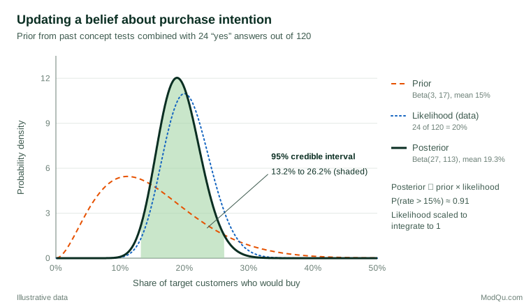
The two analyses broadly agree: the best estimate is close to 20%, and the uncertainty is wide. They differ in what they let us say. The frequentist result cannot be stated as "there is a 94% chance the true rate is above 15%", because the p-value is not the probability that a hypothesis is true (Wasserstein & Lazar, 2016). The Bayesian result can be stated in exactly those direct terms, but only conditional on the prior chosen. A manager weighing a launch will usually find the Bayesian statement easier to use; a reviewer wary of the analyst's assumptions may prefer the frequentist one.
Comparing the two approaches
| Question | Frequentist | Bayesian |
|---|---|---|
| What is probability? | Long-run frequency of events | Degree of belief given information |
| Unknown parameters | Fixed constants | Quantities with probability distributions |
| Prior information | Not formally used | Built in through the prior |
| Interval estimate | Confidence interval | Credible interval |
| Testing hypotheses | p-values, significance levels | Posterior probabilities, Bayes factors |
| Main strength | No prior needed; well-defined error rates | Direct probability statements; combines evidence |
| Main criticism | Results are easily misinterpreted | Conclusions depend on the prior |
Confidence intervals and credible intervals
The interval estimates illustrate the difference most clearly. A 95% confidence interval does not mean there is a 95% probability that the true value lies inside that particular interval. The 95% describes the method: in repeated samples, 95% of intervals constructed this way would contain the true value. Any single interval either contains it or does not. Hoekstra et al. (2014) found that most researchers and students they surveyed endorsed at least one false statement about the meaning of a confidence interval, and experienced researchers did no better than students.
A 95% credible interval means what most people assume a confidence interval means: given the prior and the data, there is a 95% probability that the true value lies within it. With large samples and weak priors, the two intervals are often numerically almost identical.
p-values and Bayes factors
Frequentist testing asks how surprising the data would be if the null hypothesis were true. Bayesian testing asks how much the data should shift belief between competing hypotheses. One Bayesian tool for this is the Bayes factor: the ratio of how well two hypotheses predict the observed data (Kass & Raftery, 1995). A Bayes factor of 10 means the data are ten times more probable under one hypothesis than under the other.
The two kinds of evidence do not always agree. Berger and Sellke (1987) showed that, when testing a precise null hypothesis, a p-value of 0.05 can correspond to a substantial posterior probability that the null is true, so p-values may overstate the evidence against it. Casella and Berger (1987) showed that for one-sided tests, by contrast, the two approaches can be reconciled much more closely. Wagenmakers (2007) reviews the problems with p-values from a Bayesian perspective and proposes a practical approximation to the Bayes factor. The broader lesson, stressed in the American Statistical Association's statement, is that no single number should decide a business or scientific conclusion (Wasserstein & Lazar, 2016).
The role and risk of the prior
The prior is both the greatest strength and the most criticised feature of Bayesian analysis. Efron (1986) argued that the difficulty of specifying priors objectively is the main reason frequentist methods remained dominant in scientific reporting. A badly chosen prior can pull estimates towards the analyst's expectations.
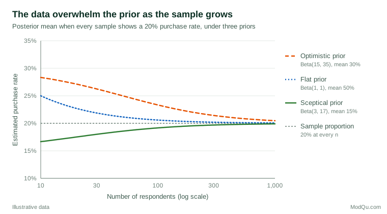
Three points soften this concern. First, as the sample grows, the data dominate any reasonable prior, so analysts who begin with different priors converge on the same answer (Figure 2). Second, priors can be weakly informative, ruling out only implausible values, and they should be judged together with the model and data they are combined with rather than in isolation (Gelman et al., 2017). Third, good Bayesian practice includes checking whether the model and prior produce predictions that resemble the real data, and revising them if not (Gelman & Shalizi, 2013).
Practical guidance for survey and business data
For large, well-designed surveys, both methods give very similar estimates, and the choice matters less than sample and question quality. They differ most in these situations.
- Small samples and subgroups. When estimates are needed for small regions, niche segments or rare customer types, Bayesian hierarchical models "borrow strength" across groups and give more stable estimates than analysing each group alone (Gelman et al., 2013).
- Non-representative samples. Bayesian multilevel regression and poststratification can adjust opt-in survey data to population targets. Wang et al. (2015) used it to produce reasonable election forecasts from a highly unrepresentative online poll.
- Repeated studies. Tracking studies and concept tests that recur can use earlier waves as prior information, rather than treating each wave as if nothing were known.
- Decisions under uncertainty. When the question is "how likely is it that this option is better?", posterior probabilities answer it directly and feed naturally into cost and benefit calculations (Kruschke & Liddell, 2018).
- Regulated or adversarial settings. Where results must be defended against critics, frequentist methods with pre-specified error rates, or Bayesian analyses with sceptical and pre-registered priors, reduce the suspicion that assumptions were tuned to the desired answer.
Many statisticians now take a pragmatic position. Bayarri and Berger (2004) describe how each school borrows from and improves the other. Little (2006) proposes "calibrated Bayes": use Bayesian methods for inference, and use frequentist ideas to check that those methods perform well over repeated use.
Common mistakes
- Reading a p-value as the probability that the null hypothesis is true. It is not, and treating p = 0.06 as "no effect" or p = 0.04 as "proven" misreads it in both directions (Greenland et al., 2016).
- Interpreting a confidence interval as a credible interval. The direct probability statement belongs only to the Bayesian interval.
- Hiding the prior. A Bayesian analysis should state its prior, explain where it came from and show how much the conclusions change under alternatives.
- Choosing the prior after seeing the data. This defeats its purpose and can produce almost any result.
- Treating the debate as a reason to ignore uncertainty. Both schools agree that estimates should be reported with a measure of their precision.
Key takeaways
Frequentist statistics treats probability as long-run frequency and judges methods by how they perform over repeated samples. Bayesian statistics treats probability as a degree of belief and updates prior knowledge with data to give direct probability statements about unknown quantities. With large samples the two usually agree; with small samples, prior information or decisions that need a probability of success, the Bayesian approach often adds value, provided its assumptions are stated openly. The most useful habit for any analyst or reader is to know which question a reported number answers.
References
Bayarri, M. J., & Berger, J. O. (2004). The interplay of Bayesian and frequentist analysis. Statistical Science, 19(1), 58–80. https://doi.org/10.1214/088342304000000116
Bayes, T. (1763). An essay towards solving a problem in the doctrine of chances. Philosophical Transactions of the Royal Society of London, 53, 370–418. https://doi.org/10.1098/rstl.1763.0053
Berger, J. O., & Sellke, T. (1987). Testing a point null hypothesis: The irreconcilability of P values and evidence. Journal of the American Statistical Association, 82(397), 112–122. https://doi.org/10.1080/01621459.1987.10478397
Casella, G., & Berger, R. L. (1987). Reconciling Bayesian and frequentist evidence in the one-sided testing problem. Journal of the American Statistical Association, 82(397), 106–111. https://doi.org/10.1080/01621459.1987.10478396
Edwards, W., Lindman, H., & Savage, L. J. (1963). Bayesian statistical inference for psychological research. Psychological Review, 70(3), 193–242. https://doi.org/10.1037/h0044139
Efron, B. (1986). Why isn't everyone a Bayesian? The American Statistician, 40(1), 1–5. https://doi.org/10.1080/00031305.1986.10475342
Fisher, R. A. (1922). On the mathematical foundations of theoretical statistics. Philosophical Transactions of the Royal Society of London. Series A, Containing Papers of a Mathematical or Physical Character, 222(594–604), 309–368. https://doi.org/10.1098/rsta.1922.0009
Gelman, A., Carlin, J. B., Stern, H. S., Dunson, D. B., Vehtari, A., & Rubin, D. B. (2013). Bayesian data analysis (3rd ed.). Chapman and Hall/CRC. https://doi.org/10.1201/b16018
Gelman, A., & Shalizi, C. R. (2013). Philosophy and the practice of Bayesian statistics. British Journal of Mathematical and Statistical Psychology, 66(1), 8–38. https://doi.org/10.1111/j.2044-8317.2011.02037.x
Gelman, A., Simpson, D., & Betancourt, M. (2017). The prior can often only be understood in the context of the likelihood. Entropy, 19(10), Article 555. https://doi.org/10.3390/e19100555
Greenland, S., Senn, S. J., Rothman, K. J., Carlin, J. B., Poole, C., Goodman, S. N., & Altman, D. G. (2016). Statistical tests, P values, confidence intervals, and power: A guide to misinterpretations. European Journal of Epidemiology, 31(4), 337–350. https://doi.org/10.1007/s10654-016-0149-3
Hoekstra, R., Morey, R. D., Rouder, J. N., & Wagenmakers, E.-J. (2014). Robust misinterpretation of confidence intervals. Psychonomic Bulletin & Review, 21(5), 1157–1164. https://doi.org/10.3758/s13423-013-0572-3
Kass, R. E., & Raftery, A. E. (1995). Bayes factors. Journal of the American Statistical Association, 90(430), 773–795. https://doi.org/10.1080/01621459.1995.10476572
Kruschke, J. K., & Liddell, T. M. (2018). The Bayesian New Statistics: Hypothesis testing, estimation, meta-analysis, and power analysis from a Bayesian perspective. Psychonomic Bulletin & Review, 25(1), 178–206. https://doi.org/10.3758/s13423-016-1221-4
Lindley, D. V. (2000). The philosophy of statistics. Journal of the Royal Statistical Society: Series D (The Statistician), 49(3), 293–337. https://doi.org/10.1111/1467-9884.00238
Little, R. J. (2006). Calibrated Bayes: A Bayes/frequentist roadmap. The American Statistician, 60(3), 213–223. https://doi.org/10.1198/000313006X117837
McElreath, R. (2020). Statistical rethinking: A Bayesian course with examples in R and Stan (2nd ed.). Chapman and Hall/CRC. https://doi.org/10.1201/9780429029608
Neyman, J. (1937). Outline of a theory of statistical estimation based on the classical theory of probability. Philosophical Transactions of the Royal Society of London. Series A, Mathematical and Physical Sciences, 236(767), 333–380. https://doi.org/10.1098/rsta.1937.0005
Neyman, J., & Pearson, E. S. (1933). On the problem of the most efficient tests of statistical hypotheses. Philosophical Transactions of the Royal Society of London. Series A, Containing Papers of a Mathematical or Physical Character, 231(694–706), 289–337. https://doi.org/10.1098/rsta.1933.0009
Wagenmakers, E.-J. (2007). A practical solution to the pervasive problems of p values. Psychonomic Bulletin & Review, 14(5), 779–804. https://doi.org/10.3758/BF03194105
Wang, W., Rothschild, D., Goel, S., & Gelman, A. (2015). Forecasting elections with non-representative polls. International Journal of Forecasting, 31(3), 980–991. https://doi.org/10.1016/j.ijforecast.2014.06.001
Wasserstein, R. L., & Lazar, N. A. (2016). The ASA statement on p-values: Context, process, and purpose. The American Statistician, 70(2), 129–133. https://doi.org/10.1080/00031305.2016.1154108