
Statistics · Distributions
Extreme Value Theory Applications for Tail Risk Knowledge
How extreme value theory estimates the size and frequency of rare, damaging events, from block maxima to peaks over threshold, with a worked insurance example and practical guidance for business risk.
Most statistical tools describe the middle of a distribution: the average order, the typical rating, the usual week. Many business decisions, however, turn on the edges. How large could the worst insurance claim of the decade be? What demand spike should a call centre or warehouse be able to absorb? How much capital covers a 1-in-200-year loss? These questions are about the tail of a distribution, the region where data are scarce and ordinary models are least reliable.
Extreme value theory (EVT) is the branch of statistics built for these questions. Instead of fitting one model to all the data and hoping it holds in the tail, EVT uses limit theorems that describe how the largest values behave, whatever the shape of the distribution in its middle. It is used to set flood defences, price reinsurance and measure market and operational risk in banks (Coles, 2001; Embrechts et al., 1997). This article explains the two main approaches, works through a hypothetical insurance example, and sets out the practical choices and mistakes that matter most.
Why ordinary models fail in the tail
A model fitted to an entire dataset is judged mostly by how well it matches the bulk of the observations, because that is where most of the data lie. Small misfits in the tail barely affect the overall fit, yet they can change estimates of rare events by a factor of two or more. The normal distribution is the usual culprit. Its tails fall away so quickly that a value five standard deviations above the mean should occur less than once in three million observations. Financial returns, insurance losses, project overruns and many demand series produce such values far more often.
The core difficulty is that rare events are, by definition, rarely observed. A dataset of 5,000 claims contains about five that exceed its own 99.9th percentile, and nothing at all about what lies beyond its largest value. Estimating a 1-in-1,000 or 1-in-10,000 event therefore requires extrapolation: going beyond the observed range. EVT does not remove that problem, but it puts the extrapolation on a theoretical footing and attaches honest uncertainty to it.
The theory in brief
Block maxima and the generalised extreme value distribution
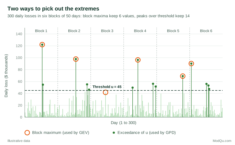
The classical result concerns the largest value in a block of observations, such as the highest daily loss in each year. Fisher and Tippett (1928) showed that, after suitable rescaling, such maxima can converge to only three types of limiting distribution, and Gnedenko (1943) gave the conditions under which each applies. The three types are now known as the Gumbel, Fréchet and Weibull families, after the researchers who studied them; Gumbel (1958) popularised their use for floods and other practical problems. Jenkinson (1955) combined all three into one formula, the generalised extreme value (GEV) distribution:
G(z) = exp{ −[1 + ξ(z − μ) ÷ σ]−1/ξ }
Here μ is a location parameter, σ a scale parameter and ξ (xi) the shape parameter, which controls the tail. When ξ > 0 the tail is heavy, decaying like a power law, as in many financial and insurance losses. When ξ = 0 (the Gumbel case, taken as a limit) the tail decays exponentially, as for the normal and lognormal distributions. When ξ < 0 there is a finite upper limit, as for quantities with a physical cap. The GEV plays a role for maxima similar to that of the normal distribution for averages under the central limit theorem.
Peaks over threshold and the generalised Pareto distribution
Keeping only one maximum per block wastes information. A bad year may contain several large losses, while a quiet year contributes its largest value even if it is unremarkable. The alternative, peaks over threshold (POT), keeps every observation that exceeds a high threshold u. Balkema and de Haan (1974) and Pickands (1975) showed that, for a wide class of distributions, the excesses over a sufficiently high threshold follow approximately a generalised Pareto distribution (GPD):
H(y) = 1 − (1 + ξy ÷ σu)−1/ξ, y = x − u > 0
The shape parameter ξ is the same one that appears in the GEV, so the two approaches tell a consistent story about the tail. Davison and Smith (1990) developed the POT method into a full modelling framework, including covariates and diagnostics, and it is now the more common choice in insurance and finance because it uses the scarce tail data more efficiently.
What the shape parameter means in practice
The shape parameter is the single most important output of an EVT analysis. A positive ξ means the tail follows a power law, and the moments of order 1/ξ and higher do not exist. With ξ = 0.5, for example, the variance is infinite; with ξ ≥ 1 even the mean is infinite. Such tails make sample averages unstable and make the largest observations dominate totals. The tail index α = 1/ξ is often estimated directly with the estimator of Hill (1975), which uses the logarithms of the k largest observations. It is simple, but its value can shift considerably with the choice of k, and Drees et al. (2000) discuss why the familiar "Hill plot" of estimates against k is often hard to read.
Measuring tail risk
EVT is usually a means to an end: an estimate of a quantity that decision-makers need. Three are common.
- Return levels. The T-period return level is the value exceeded on average once every T periods. A 100-year flood level, or the 1-in-50-year peak week of demand, is a return level. It is an average frequency, not a schedule: a 100-year event can occur in consecutive years.
- Value at risk (VaR). The VaR at level p is the p-quantile of the loss distribution, for example the 99.5% quantile of annual losses used in insurance solvency calculations.
- Expected shortfall (ES). The expected shortfall is the average loss given that the VaR is exceeded. It tells you how bad things are when the bad day arrives. Artzner et al. (1999) showed that VaR can fail to reward diversification, because the VaR of a combined portfolio can exceed the sum of its parts, whereas expected shortfall belongs to a class of "coherent" risk measures that do not have this flaw. The Basel Committee on Banking Supervision (2019) accordingly moved its market risk standard from a 99% VaR to a 97.5% expected shortfall.
Under the POT model, with N observations of which Nu exceed the threshold, both measures have closed forms (McNeil & Frey, 2000):
VaRp = u + (σu ÷ ξ) × { [(N ÷ Nu)(1 − p)]−ξ − 1 }
ESp = VaRp ÷ (1 − ξ) + (σu − ξu) ÷ (1 − ξ), for ξ < 1
A worked example: sizing large insurance claims
Suppose a hypothetical insurer holds 5,000 property claims. The mean claim is about $9,600, the median about $5,100, and the standard deviation about $14,700. The largest claim is just under $300,000. Management wants to know how large a 1-in-1,000 claim is likely to be, to set a reinsurance retention, and what the average claim beyond that point would cost. (The data were simulated from a known heavy-tailed distribution, which lets us check the answers.)
Step 1: choose a threshold. We set u at the 95th percentile, about $33,000, leaving 250 exceedances. A higher threshold would make the GPD approximation more accurate but leave fewer data; a lower one would add data but risk bias. Checking the choice is discussed below.
Step 2: fit the GPD to the excesses. Maximum likelihood gives ξ ≈ 0.29 and σu ≈ $16,600. The positive shape confirms a heavy, power-law tail. Smith (1985) showed that maximum likelihood behaves regularly when ξ > −0.5, which covers almost all practical loss data. For small samples, the probability-weighted moment estimators of Hosking et al. (1985) and Hosking and Wallis (1987) are useful alternatives.
Step 3: compute the risk measures. Applying the formulas gives the results in the table, alongside what a normal distribution fitted to all 5,000 claims would say.
| Measure | Generalised Pareto tail | Normal distribution | Sample (empirical) |
|---|---|---|---|
| 99% quantile (1 in 100) | $67,000 | $44,000 | $67,000 |
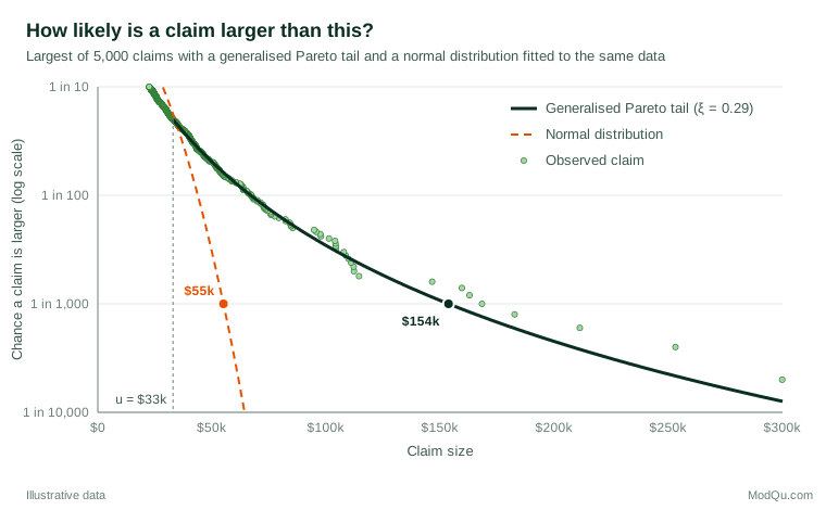
| 99.9% quantile (1 in 1,000) | $154,000 | $55,000 | $163,000 |
| Expected shortfall at 99.9% | $226,000 | $59,000 | based on 5 claims |
At the 1-in-100 level, where data are still plentiful, the GPD and the sample agree closely, while the normal model is already a third too low. At the 1-in-1,000 level, the normal model suggests $55,000; the GPD suggests $154,000, almost three times as much. Figure 2 shows why: on a log-probability scale, the observed large claims follow the GPD curve, while the normal curve plunges away from them.
Step 4: state the uncertainty. A bootstrap of the 250 exceedances gives an approximate 95% interval for the 1-in-1,000 claim of $125,000 to $187,000. Because the data were simulated, we know the true value is $180,000: inside the interval but above the point estimate. That is typical. Tail estimates are uncertain, and the uncertainty is lopsided, with more room above the estimate than below. Profile likelihood intervals, which respect this asymmetry, are generally preferred to symmetric "plus or minus" intervals (Coles, 2001).
Step 5: check alternatives. For comparison, Hill estimates of the tail index α range from about 2.6 using the top 100 claims to 2.0 using the top 500, against a true value of 3. This sensitivity to k is a reminder that no single tail number should be reported without showing how it moves with modelling choices.
Applications beyond insurance
Finance. McNeil and Frey (2000) combined a volatility model with a POT fit to the standardised residuals, so that tail estimates respond to calm and turbulent periods. Danielsson and de Vries (1997) applied tail index methods to high-frequency trading data. Both approaches underpin many market risk systems.
Operational and catastrophe losses. McNeil (1997) used EVT on large Danish fire insurance losses and showed how strongly tail estimates depend on threshold choice. Similar models are used for fraud losses, IT outages and cyber incidents, where a few events dominate annual totals.
Environment and infrastructure. Hydrology and climate science are the oldest users of extremes methods, from flood return levels to rainfall intensity (Katz et al., 2002). Businesses use these results when siting warehouses, data centres and stores, and when assessing supply chain exposure to storms or heatwaves.
Operations and demand. Peak daily orders, call volumes and delivery delays have tails that drive capacity costs. A return-level analysis states how often planned capacity is expected to be exceeded.
Survey and customer data. Distributions of income, wealth and spending are typically skewed with long upper tails, and the very largest values are often top-coded, missing or under-represented in samples. Fitting a Pareto-type tail to the upper part of such distributions is a common way to model the top end. In customer analytics, a small number of very high-value customers can account for a large share of revenue, and EVT helps judge whether a model of "whale" behaviour is plausible. When a dataset is said to follow a power law, the tests of Clauset et al. (2009) help check whether that claim is supported or whether another heavy-tailed distribution fits as well.
Practical guidance
Choosing the threshold or block size
Threshold choice is the central practical decision in POT analysis, and it is a bias–variance trade-off. Standard diagnostics include the mean residual life plot, which should become roughly linear above a suitable threshold, and plots of the estimated shape parameter across a range of thresholds, which should be roughly stable above it (Coles, 2001). Report results for several thresholds. For block maxima, blocks must be long enough for the GEV approximation to hold but numerous enough to estimate three parameters; annual blocks are common for environmental data.
Dealing with clusters and trends
The basic theory assumes independent observations. Real extremes often cluster: one storm produces several days of high claims, and one market shock produces a run of large losses. Leadbetter et al. (1983) extended the theory to dependent sequences through the extremal index, which measures the degree of clustering, and Ferro and Segers (2003) provided methods for estimating it. In practice, analysts often decluster by keeping only the peak of each cluster. Trends, such as growing claim sizes from inflation or a changing climate, should be modelled explicitly, for example by letting the GEV or GPD parameters depend on time (Davison & Smith, 1990).
Software and reporting
Mature software is widely available; Gilleland and Katz (2016) describe one well-documented package that covers GEV and GPD fitting, diagnostics and non-stationary models. Whatever tool is used, a report should state the threshold or block size, the number of exceedances, the estimated shape with its interval, the diagnostic plots, and the sensitivity of the key estimate to these choices. Several textbooks give fuller guidance (Beirlant et al., 2004; de Haan & Ferreira, 2006).
Limitations and common mistakes
- Treating extrapolation as certainty. EVT justifies the shape of the tail, not the precision of any number far beyond the data. A 1-in-10,000 estimate from 20 years of data rests heavily on the model.
- Using too little tail data. With fewer than about 50 exceedances or blocks, shape estimates become very unstable.
- Ignoring dependence and change. Clustered or trending data violate the basic assumptions and usually make naive estimates too optimistic.
- Reporting only VaR. A quantile says nothing about how large losses are beyond it. Pair it with expected shortfall, and note that expected shortfall does not exist when ξ ≥ 1.
- Fitting the whole distribution and reading off the tail. This is exactly the practice EVT replaces. A lognormal or normal model chosen for the bulk can understate tail risk severely, as the worked example shows.
- Forgetting that the data-generating process can change. New products, policies or markets can create tails that past data never showed. EVT should be combined with scenario analysis and expert judgement, not used in place of them.
Key takeaways
Extreme value theory gives a principled way to estimate events that are rarer than anything a dataset contains. The block maxima approach fits the generalised extreme value distribution to periodic maxima; the peaks-over-threshold approach fits the generalised Pareto distribution to all large values and usually makes better use of scarce data. The shape parameter ξ summarises how heavy the tail is and drives every downstream estimate. Used with careful threshold choice, attention to clustering and trends, and honest, asymmetric uncertainty intervals, EVT turns questions about rare losses, demand peaks and extreme customers into quantities that can be planned for. Its central lesson for business is simple: do not let a model built for the average decide how bad the worst case can be.
References
Artzner, P., Delbaen, F., Eber, J.-M., & Heath, D. (1999). Coherent measures of risk. Mathematical Finance, 9(3), 203–228. https://doi.org/10.1111/1467-9965.00068
Balkema, A. A., & de Haan, L. (1974). Residual life time at great age. The Annals of Probability, 2(5), 792–804. https://doi.org/10.1214/aop/1176996548
Basel Committee on Banking Supervision. (2019). Minimum capital requirements for market risk. Bank for International Settlements. https://www.bis.org/bcbs/publ/d457.htm
Beirlant, J., Goegebeur, Y., Segers, J., & Teugels, J. (2004). Statistics of extremes: Theory and applications. Wiley. https://doi.org/10.1002/0470012382
Clauset, A., Shalizi, C. R., & Newman, M. E. J. (2009). Power-law distributions in empirical data. SIAM Review, 51(4), 661–703. https://doi.org/10.1137/070710111
Coles, S. (2001). An introduction to statistical modeling of extreme values. Springer. https://doi.org/10.1007/978-1-4471-3675-0
Danielsson, J., & de Vries, C. G. (1997). Tail index and quantile estimation with very high frequency data. Journal of Empirical Finance, 4(2–3), 241–257. https://doi.org/10.1016/S0927-5398(97)00008-X
Davison, A. C., & Smith, R. L. (1990). Models for exceedances over high thresholds. Journal of the Royal Statistical Society Series B: Statistical Methodology, 52(3), 393–425. https://doi.org/10.1111/j.2517-6161.1990.tb01796.x
de Haan, L., & Ferreira, A. (2006). Extreme value theory: An introduction. Springer. https://doi.org/10.1007/0-387-34471-3
Drees, H., de Haan, L., & Resnick, S. (2000). How to make a Hill plot. The Annals of Statistics, 28(1), 254–274. https://doi.org/10.1214/aos/1016120372
Embrechts, P., Klüppelberg, C., & Mikosch, T. (1997). Modelling extremal events for insurance and finance. Springer. https://doi.org/10.1007/978-3-642-33483-2
Ferro, C. A. T., & Segers, J. (2003). Inference for clusters of extreme values. Journal of the Royal Statistical Society Series B: Statistical Methodology, 65(2), 545–556. https://doi.org/10.1111/1467-9868.00401
Fisher, R. A., & Tippett, L. H. C. (1928). Limiting forms of the frequency distribution of the largest or smallest member of a sample. Mathematical Proceedings of the Cambridge Philosophical Society, 24(2), 180–190. https://doi.org/10.1017/S0305004100015681
Gilleland, E., & Katz, R. W. (2016). extRemes 2.0: An extreme value analysis package in R. Journal of Statistical Software, 72(8), 1–39. https://doi.org/10.18637/jss.v072.i08
Gnedenko, B. (1943). Sur la distribution limite du terme maximum d'une série aléatoire. Annals of Mathematics, 44(3), 423–453. https://doi.org/10.2307/1968974
Gumbel, E. J. (1958). Statistics of extremes. Columbia University Press. https://doi.org/10.7312/gumb92958
Hill, B. M. (1975). A simple general approach to inference about the tail of a distribution. The Annals of Statistics, 3(5), 1163–1174. https://doi.org/10.1214/aos/1176343247
Hosking, J. R. M., & Wallis, J. R. (1987). Parameter and quantile estimation for the generalized Pareto distribution. Technometrics, 29(3), 339–349. https://doi.org/10.1080/00401706.1987.10488243
Hosking, J. R. M., Wallis, J. R., & Wood, E. F. (1985). Estimation of the generalized extreme-value distribution by the method of probability-weighted moments. Technometrics, 27(3), 251–261. https://doi.org/10.1080/00401706.1985.10488049
Jenkinson, A. F. (1955). The frequency distribution of the annual maximum (or minimum) values of meteorological elements. Quarterly Journal of the Royal Meteorological Society, 81(348), 158–171. https://doi.org/10.1002/qj.49708134804
Katz, R. W., Parlange, M. B., & Naveau, P. (2002). Statistics of extremes in hydrology. Advances in Water Resources, 25(8–12), 1287–1304. https://doi.org/10.1016/S0309-1708(02)00056-8
Leadbetter, M. R., Lindgren, G., & Rootzén, H. (1983). Extremes and related properties of random sequences and processes. Springer. https://doi.org/10.1007/978-1-4612-5449-2
McNeil, A. J. (1997). Estimating the tails of loss severity distributions using extreme value theory. ASTIN Bulletin, 27(1), 117–137. https://doi.org/10.2143/AST.27.1.563210
McNeil, A. J., & Frey, R. (2000). Estimation of tail-related risk measures for heteroscedastic financial time series: An extreme value approach. Journal of Empirical Finance, 7(3–4), 271–300. https://doi.org/10.1016/S0927-5398(00)00012-8
Pickands, J., III. (1975). Statistical inference using extreme order statistics. The Annals of Statistics, 3(1), 119–131. https://doi.org/10.1214/aos/1176343003
Smith, R. L. (1985). Maximum likelihood estimation in a class of nonregular cases. Biometrika, 72(1), 67–90. https://doi.org/10.1093/biomet/72.1.67